5  Rain Gauges vs Gridded Precipitation Analysis

5.1 Library

We utilize the terra package for rasters (Hijmans 2024). The package KableExtra is for table visualizations(Hao Zhu 2024). The sp package is used for calculating distances (Pebesma and Bivand 2005). Packages purr and tiblle are for data wrangling Müller and Wickham (2023)

library(dplyr)
library(terra)
library(readxl)
library(kableExtra)
library(purrr)
library(sp)
library(tibble)
library(ggplot2)

Read in files for the analysis

# Read in the data
data_ground<- read.csv("../tables/precipitation.csv")
striStation<- read.csv("../tables/stri_met_stations.csv")
acpStation<- read.csv("../data_ground/met_data/ACP_data/cleanedVV/ACP_met_stations.csv")

#Global variables
extentMap  <- terra::ext(c(-80.2,-79.4, 8.8, 9.5))

5.2 Functions

calculate_climatology<- function(minyear,maxyear,data){
    climatology<- data %>% 
        dplyr::select(year,site,annual,jfma,gap_fill)%>%
        filter(year>=minyear&year<=maxyear)%>%
        group_by(site)%>%
        summarize(annual=mean(annual,na.rm=TRUE),
                jfma=mean(jfma,na.rm=TRUE),
                gapFill_percentage = mean(gap_fill, na.rm = TRUE) * 100)
    return(climatology)
}

annual_pan<-function(list,extent){
  b<-terra::rast(list)
  c<-terra::app(b,sum)
  d<-terra::crop(c,extent)
  return(d)
}

jfma_pan <- function(list, extent) {
  b <- terra::rast(head(list, 4))
  c <- terra::app(b, sum)
  d <- terra::crop(c, extent)
  return(d)
}

find_nearest_non_na <- function(raster_object, coordinate) {
  non_na_cells <- which(!is.na(terra::values(raster_object)))
  non_na_coords <- xyFromCell(raster_object, non_na_cells)
  dists <- sp::spDists(x = matrix(coordinate, nrow = 1), y = non_na_coords, longlat = TRUE)
  nearest_cell <- non_na_cells[which.min(dists)]
  return(terra::values(raster_object)[nearest_cell])
}



extract_land <- function(list_object, coordinate) {
  result <- numeric(nrow(coordinate))
  for (i in seq_len(nrow(coordinate))) {
    extracted_value <- terra::extract(list_object, coordinate[i, ], na.rm = FALSE)[1,2]
    result[i] <- ifelse(is.na(extracted_value), find_nearest_non_na(list_object, as.matrix(coordinate[i, ])), extracted_value)
  }
  return(result)
}

find_nearest_non_na_id <- function(raster_object, coordinate) {
  non_na_cells <- which(!is.na(terra::values(raster_object)))
  non_na_coords <- xyFromCell(raster_object, non_na_cells)
  dists <- sp::spDists(x = matrix(coordinate, nrow = 1), y = non_na_coords, longlat = TRUE)
  nearest_cell <- non_na_cells[which.min(dists)]
  return(nearest_cell)
}

extract_row_column <- function(list_object, coordinate) {
  result <- character(nrow(coordinate))  # Use character vector to store "row,col"
  for (i in seq_len(nrow(coordinate))) {
    extracted_value <- terra::extract(list_object, coordinate[i, ], na.rm = FALSE)[1, 2]
    extracted_id <- terra::extract(list_object, coordinate[i, ], na.rm = FALSE,cells=TRUE)[1,3]
    
    result[i] <- ifelse(is.na(extracted_value), find_nearest_non_na_id(list_object,as.matrix(coordinate[i,])), extracted_id)
    
  }
  return(result)
}


#stats calculation
stats<-function(predicted,observed){
  correlation<-cor.test(observed,predicted)$estimate
  rmse<-sqrt(mean((predicted-observed)^2 , na.rm = TRUE ) )
  bias<- mean((predicted-observed),na.rm=TRUE)
  mae<-  mean(abs(predicted-observed), na.rm = TRUE)
  done<-c(correlation,rmse,bias,mae)
  return(done)
}

List of data sets, their temporal extents and the location of the climatology tiffs for each of them

datasets_info <- list(
  list(start_year = 1979, end_year = 2013, dataset_name = "CHELSA 1.2",column_name="CHELSA1.2", temporal = "1979-2013",path = "../data_reanalysis/CHELSA 1.2/"),
  list(start_year = 1981, end_year = 2010, dataset_name = "CHELSA 2.1",column_name="CHELSA2.1", temporal = "1981-2010", path = "../data_reanalysis/CHELSA 2.1/"),
  list(start_year = 2003, end_year = 2016, dataset_name = "CHELSA EarthEnv",column_name="CHELSA_EarthEnv", temporal = "2003-2016",path = "../data_reanalysis/CHELSA EarthEnv/climatology"),
  list(start_year = 1980, end_year = 2009, dataset_name = "CHPclim",column_name="CHPclim", temporal = "1980-2009", path = "../data_reanalysis/CHPclim/"),
  list(start_year = 1970, end_year = 2000, dataset_name = "WorldClim 2.1",column_name="WorldClim2.1", temporal = "1970-2000", path = "../data_reanalysis/WorldClim 2.1"),
  list(start_year = 1981, end_year = 2016, dataset_name = "CHIRPS 2.0",column_name="CHIRPS2.0",temporal = "1981-2016", path = "../data_reanalysis/CHIRPS 2.0/climatology"),
  list(start_year = 1979, end_year = 2016, dataset_name = "CHELSA-W5E5v1.0",column_name="CHELSAW5E5v1.0", temporal = "1979-2016",path = "../data_reanalysis/CHELSA-W5E5v1.0/climatology"),
  list(start_year = 1981, end_year = 2010, dataset_name = "TerraClimate",column_name="TerraClimate", temporal = "1981-2010", path = "../data_reanalysis/TerraClimate"),
  list(start_year = 1979, end_year = 2013, dataset_name = "PBCOR CHELSA 1.2",column_name="PBCOR_CHELSA1.2", temporal = "1979-2013", path = "../data_reanalysis/PBCOR/CHELSA 1.2 corrected"),
  list(start_year = 1980, end_year = 2009, dataset_name = "PBCOR CHPclim",column_name="PBCOR_CHPclim", temporal = "1980-2009", path = "../data_reanalysis/PBCOR/CHPclim corrected"),
  list(start_year = 1970, end_year = 2000, dataset_name = "PBCOR WorldClim 2.1",column_name="PBCOR_WorldClim2.1", temporal = "1970-2000", path = "../data_reanalysis/PBCOR/WorldClim corrected")
)

5.3 Climatologies

Loop through each dataset and calculate climatology

climatologies <- datasets_info %>%
  map_df(function(info) {
    calculate_climatology(info$start_year, info$end_year, data_ground) %>%
      mutate(source = info$dataset_name)}) %>%
  left_join(acpStation[, c('site', 'latitude', 'longitude', 'Elevation')], by = c("site" = "site")) %>%
  left_join(striStation[, c('alias', 'latitude', 'longitude')], by = c("site" = "alias")) %>%
  mutate(latitude = ifelse(is.na(latitude.x), latitude.y, latitude.x),
         longitude = ifelse(is.na(longitude.x), longitude.y, longitude.x),
         longitude = -1 * abs(longitude)) %>%
  dplyr::select(site, latitude, longitude, source, annual, jfma, Elevation, gapFill_percentage)


#extract the values at the coordinates for climatologies

for (source in datasets_info) {
  files <- list.files(source$path, pattern = "\\.tif$", full.names = TRUE)
  annual_data <- annual_pan(files, extentMap)
  climatologies[[source$dataset_name]] <- extract_land(annual_data,climatologies[,3:2])
  climatologies[[paste0(source$dataset_name,"_cell")]]<-extract_row_column(annual_data,climatologies[,3:2])
  jfma_data = jfma_pan(files, extentMap)
  column_name = paste(source$dataset_name, "_jfma", sep = "")
  climatologies[[column_name]] = extract_land(jfma_data, climatologies[,3:2])

}

write.csv(climatologies,file="../tables/climatologies.csv")

#Briefly analyse the gap filling effect on site and Gridded dataset

ggplot(climatologies, aes(x = site, y = gapFill_percentage)) +
  geom_boxplot() +
  labs(title = "Gap Fill Percentage by Site",
       x = "Site",
       y = "Gap Fill Percentage (%)") +
  theme_minimal() +
  theme(axis.text.x = element_text(angle = 45, hjust = 1))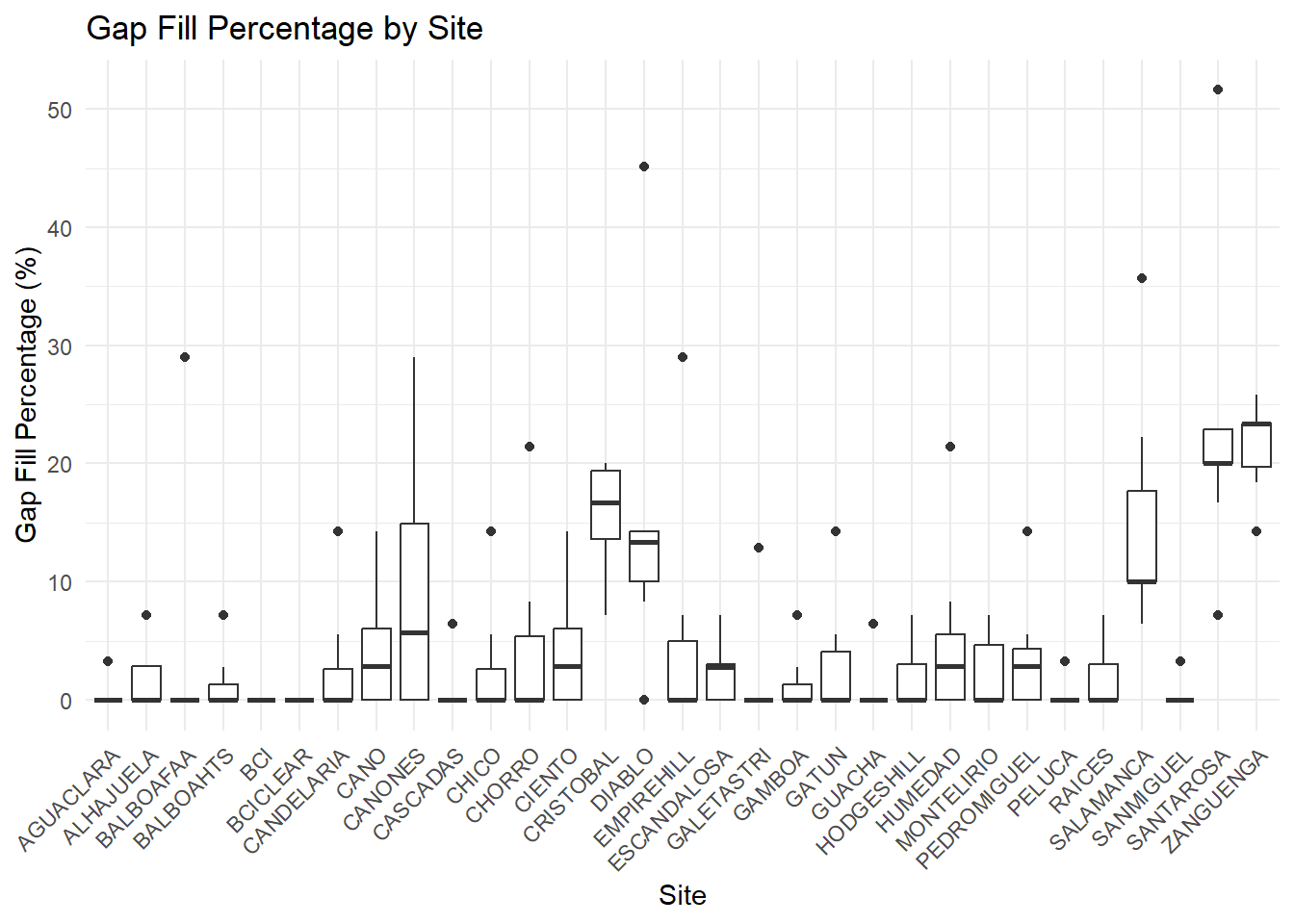

ggplot(climatologies, aes(x = source, y = gapFill_percentage)) +
  geom_boxplot() +
  labs(title = "Gap Fill Percentage by Site",
       x = "Source",
       y = "Gap Fill Percentage (%)") +
  theme_minimal() +
  theme(axis.text.x = element_text(angle = 45, hjust = 1))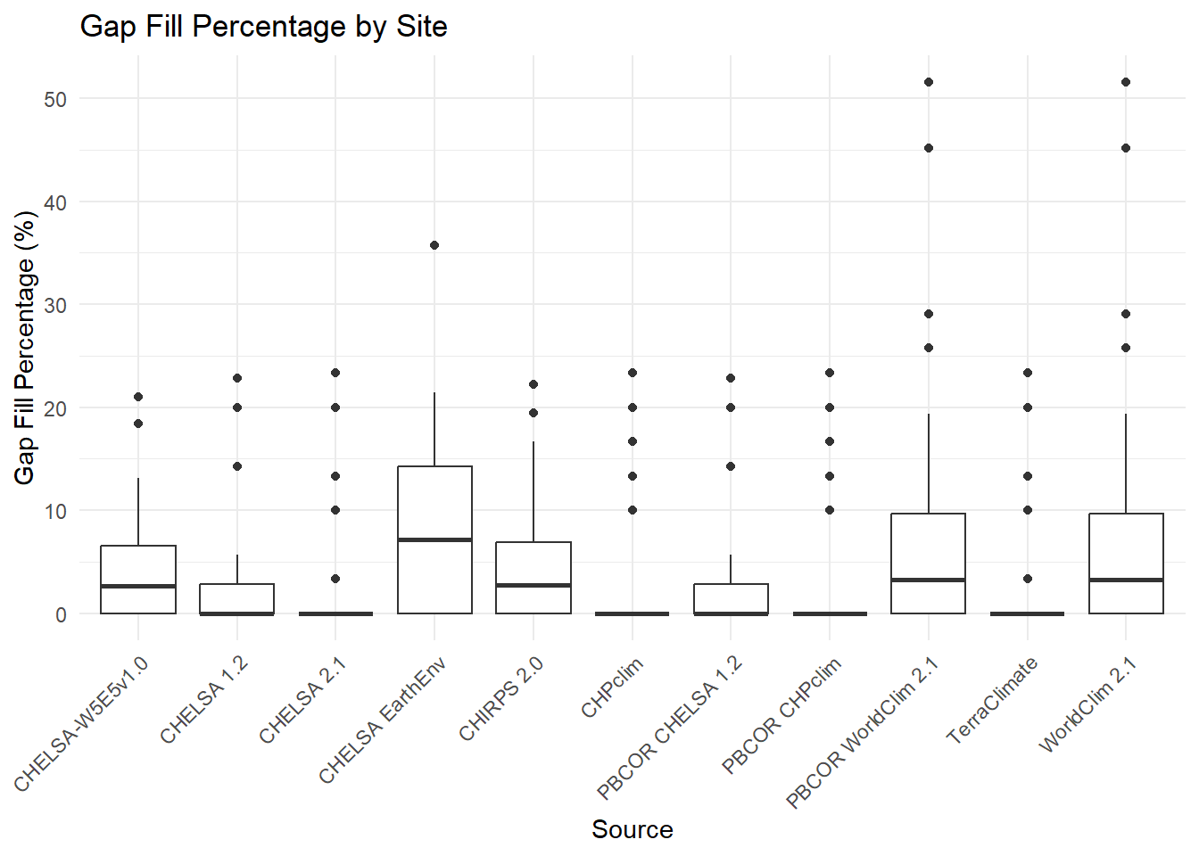

sources_unique <- unique(climatologies$source)
df<- data.frame()

for (source in sources_unique) {
  data_column <- paste0(source) 
  unique_values <- nrow(unique(climatologies[climatologies$source == source, paste0(source,"_cell")]))

  # Find sites with the same value
  sites_with_same_value <- climatologies[climatologies$source == source, ] %>%
    group_by(.data[[paste0(source, "_cell")]]) %>%                  
    filter(n() > 1) %>%             
    summarize(sites = paste(site, collapse = ", "))
  cat(paste("Source:", source, "\n"))
  cat(paste("  - Unique raster cell:", unique_values, "\n"))
  cat(paste("  - Sites in the same cell:", sites_with_same_value$sites, "\n"))
  
}

Source: CHELSA 1.2 
  - Unique raster cell: 30 
  - Sites in the same cell: BCI, BCICLEAR 
Source: CHELSA 2.1 
  - Unique raster cell: 30 
  - Sites in the same cell: BCI, BCICLEAR 
Source: CHELSA EarthEnv 
  - Unique raster cell: 30 
  - Sites in the same cell: BCI, BCICLEAR 
Source: CHPclim 
  - Unique raster cell: 28 
  - Sites in the same cell: BCI, BCICLEAR 
   - Sites in the same cell: CASCADAS, EMPIREHILL 
   - Sites in the same cell: BALBOAHTS, DIABLO 
Source: WorldClim 2.1 
  - Unique raster cell: 30 
  - Sites in the same cell: BCI, BCICLEAR 
Source: CHIRPS 2.0 
  - Unique raster cell: 28 
  - Sites in the same cell: BCI, BCICLEAR 
   - Sites in the same cell: CASCADAS, EMPIREHILL 
   - Sites in the same cell: BALBOAHTS, DIABLO 
Source: CHELSA-W5E5v1.0 
  - Unique raster cell: 30 
  - Sites in the same cell: BCI, BCICLEAR 
Source: TerraClimate 
  - Unique raster cell: 27 
  - Sites in the same cell: BCI, BCICLEAR 
   - Sites in the same cell: EMPIREHILL, HODGESHILL 
   - Sites in the same cell: BALBOAFAA, BALBOAHTS, DIABLO 
Source: PBCOR CHELSA 1.2 
  - Unique raster cell: 27 
  - Sites in the same cell: BCI, BCICLEAR 
   - Sites in the same cell: CASCADAS, EMPIREHILL 
   - Sites in the same cell: BALBOAHTS, DIABLO 
   - Sites in the same cell: CRISTOBAL, GALETASTRI 
Source: PBCOR CHPclim 
  - Unique raster cell: 28 
  - Sites in the same cell: BCI, BCICLEAR 
   - Sites in the same cell: CASCADAS, EMPIREHILL 
   - Sites in the same cell: BALBOAHTS, DIABLO 
Source: PBCOR WorldClim 2.1 
  - Unique raster cell: 27 
  - Sites in the same cell: BCI, BCICLEAR 
   - Sites in the same cell: CASCADAS, EMPIREHILL 
   - Sites in the same cell: BALBOAHTS, DIABLO 
   - Sites in the same cell: CRISTOBAL, GALETASTRI 

Compute a results data frame

results <- data.frame(
  Source = character(),
  Correlation = numeric(),
  RMSE = numeric(),
  Bias = numeric(),
  MAE = numeric(),
  stringsAsFactors = FALSE
)
results_jfma <-results

for (i in 1:length(datasets_info)) {
  source <- datasets_info[[i]]$dataset_name
  predicted <- climatologies[climatologies$source == source,][[source]]
  observed <- climatologies[climatologies$source == source,][["annual"]]
  stats_result <- stats(predicted, observed)
  
  results <- rbind(results, data.frame(
    Source = source,
    Correlation = stats_result[1],
    RMSE = stats_result[2],
    MAE = stats_result[4],
    Bias = stats_result[3],
    stringsAsFactors = FALSE
  ))
}

for (i in 1:length(datasets_info)) {
  source <- datasets_info[[i]]$dataset_name
  column=paste0(source,"_jfma")
  predicted <- climatologies[climatologies$source == source,][[column]]
  observed <- climatologies[climatologies$source == source,][["jfma"]]
  stats_result <- stats(predicted, observed)
  
  results_jfma <- rbind(results_jfma, data.frame(
    Source = source,
    Correlation = stats_result[1],
    RMSE = stats_result[2],
    MAE = stats_result[4],
    Bias = stats_result[3],
    stringsAsFactors = FALSE
  ))
}

results$Source[results$Source == "CHIRPS 2.0"] <- "CHIRPS v2.0"
results$Source[results$Source == "CHPclim"] <- "CHPclim v1.0"
results_jfma$Source[results_jfma$Source == "CHIRPS 2.0"] <- "CHIRPS v2.0"
results_jfma$Source[results_jfma$Source == "CHPclim"] <- "CHPclim v1.0"

order_vec <- c("CHELSA 1.2","CHELSA 2.1","CHELSA EarthEnv","CHELSA-W5E5v1.0","CHIRPS v2.0","CHPclim v1.0",
  "TerraClimate","WorldClim 2.1","PBCOR CHELSA 1.2","PBCOR CHPclim","PBCOR WorldClim 2.1")

results <- results[match(order_vec, results$Source), ]
results_jfma <- results_jfma[match(order_vec, results_jfma$Source), ]

#save both results as csv in tables folder
write.csv(results, file= "../tables/spatial_variation_annual.csv")
write.csv(results_jfma, file= "../tables/spatial_variation_jfma.csv")

Tables for visualizations

annual_table<-results %>%mutate(Correlation = round(Correlation, 2), RMSE= round(RMSE,0),Bias=round(Bias,0),MAE=round(MAE,0)) %>% 
  rownames_to_column(var = "rowname") %>%
  dplyr::select(-rowname) %>%
  rename("Gridded Climate Product" = "Source") %>% rename("Mean bias (mm)"="Bias")%>%
  kbl(caption = "Spatial variation among 31 sites in total annual precipitation") %>%
  kable_classic(full_width = F)
annual_table%>%save_kable("../plots/spatial_annual_variation.png",density=900)
annual_table

Spatial variation among 31 sites in total annual precipitation

Gridded Climate Product	Correlation	RMSE	MAE	Mean bias (mm)
CHELSA 1.2	0.82	310	250	53
CHELSA 2.1	0.87	475	438	390
CHELSA EarthEnv	0.85	318	258	68
CHELSA-W5E5v1.0	0.36	497	401	-19
CHIRPS v2.0	0.88	273	222	92
CHPclim v1.0	0.86	371	326	245
TerraClimate	0.78	412	346	-50
WorldClim 2.1	0.65	402	330	-24
PBCOR CHELSA 1.2	0.75	377	306	107
PBCOR CHPclim	0.77	547	463	413
PBCOR WorldClim 2.1	0.56	423	337	-21

jfma_table<-results_jfma %>%mutate(Correlation = round(Correlation, 2), RMSE= round(RMSE,0),Bias=round(Bias,0),MAE=round(MAE,0)) %>% 
  rownames_to_column(var = "rowname") %>%
  dplyr::select(-rowname) %>%
  rename("Gridded Climate Product" = "Source") %>% rename("Mean bias (mm)"="Bias")%>%
  kbl(caption = "Spatial variation among 31 sites in January-to-April precipitation") %>%
  kable_classic(full_width = F)
jfma_table%>%save_kable("../plots/spatial_jfma_variation.png",density=900)
jfma_table

Spatial variation among 31 sites in January-to-April precipitation

Gridded Climate Product	Correlation	RMSE	MAE	Mean bias (mm)
CHELSA 1.2	0.63	107	63	-35
CHELSA 2.1	0.61	105	69	-6
CHELSA EarthEnv	0.66	91	61	4
CHELSA-W5E5v1.0	0.15	125	83	-10
CHIRPS v2.0	0.82	81	49	-22
CHPclim v1.0	0.86	91	57	-46
TerraClimate	0.84	112	74	-64
WorldClim 2.1	0.47	121	84	-52
PBCOR CHELSA 1.2	0.60	108	66	-32
PBCOR CHPclim	0.81	89	54	-32
PBCOR WorldClim 2.1	0.32	131	93	-57

5.4 Seasonal variation(12-month)

month <- read.csv("../tables/monthly_ground.csv")
sites <- read.csv("../tables/dfprecip.csv")

#Filter data based on conditions
acp38 <- month %>%
  filter(site %in% c("AGUACLARA", "SANMIGUEL", "BCI", "PELUCA", "BCICLEAR", "GUACHA", "CASCADAS", "PEDROMIGUEL", "GAMBOA") & 
           Year >= 1970 & Year <= 2016) %>%
  mutate(monthlyPrecip = as.numeric(monthlyPrecip))

acp38_full_extent <- acp38 %>%
  group_by(site, Month) %>%
  summarise(mon_mean = mean(monthlyPrecip, na.rm = TRUE)) %>%
  mutate(temporal = "1970-2016", dataset_name = "Ground")

# Calculate climatology of the ground data for every specific temporal extent
acp38_ag <- lapply(datasets_info, function(dataset) {
  acp38 %>%
    filter(Year >= dataset$start_year & Year <= dataset$end_year) %>%
    group_by(site, Month) %>%
    summarise(mon_mean = mean(monthlyPrecip, na.rm = TRUE)) %>%
    mutate(temporal = dataset$temporal, dataset_name = dataset$dataset_name)
}) %>% bind_rows()

# Combine the two data frames
acp38_ag <- bind_rows(acp38_ag, acp38_full_extent)

#calculate climatology of the ground data  for every specific temporal extent

# Match lat and long
acp38_ag$long_dd <- sites$long_dd[match(acp38_ag$site, sites$site)]
acp38_ag$lat_dd <- sites$lat_dd[match(acp38_ag$site, sites$site)]


## loop for extraction of values of raster reanalyis climatologies for specific sites and month.
for (i in 1:length(datasets_info)) {
  files_list <- list.files(datasets_info[[i]]$path, pattern = "\\.tif$", full.names = TRUE)
  raster_stack <- terra::rast(files_list)
  acp38_ag[[datasets_info[[i]]$column_name]] <- NA
  for (j in 1:12) {
    acp38_ag[acp38_ag$Month == j, datasets_info[[i]]$column_name] <- extract_land(raster_stack[[j]], acp38_ag[acp38_ag$Month == j, c("long_dd", "lat_dd")])
  }
}
write.csv(acp38_ag,"../tables/acp38_ag.csv")

After extracting values, we can run some statistics

sites_unique <- unique(acp38_ag$site)
all_correlations <- data.frame( site = character(),
                                dataset=character(),
                                Correlation = numeric(),
                                RMSE = numeric(),
                                stringsAsFactors = FALSE)

#loop over the dataset and each of the sites for calculating the correlation and the rmse
for (j in seq_along(datasets_info)){
  print(datasets_info[[j]]$dataset_name)
  for (i in seq_along(sites_unique))  {
    temporal_range <- datasets_info[[j]]$temporal
    name <- datasets_info[[j]]$dataset_name
    col_name <- datasets_info[[j]]$column_name
    site_data <- acp38_ag[acp38_ag$site == sites_unique[i] & acp38_ag$temporal == temporal_range & acp38_ag$dataset_name==name, ]
    cor_test_result <- cor.test(site_data$mon_mean, unlist(site_data[,col_name]))$estimate
    rmse<-sqrt(mean(unlist(site_data[,col_name])-site_data$mon_mean)^2)
    new_row <- data.frame(site = sites_unique[i], dataset = name, Correlation = cor_test_result, RMSE = rmse)
    all_correlations <- rbind(all_correlations, new_row)
  }
}

[1] "CHELSA 1.2"
[1] "CHELSA 2.1"
[1] "CHELSA EarthEnv"
[1] "CHPclim"
[1] "WorldClim 2.1"
[1] "CHIRPS 2.0"
[1] "CHELSA-W5E5v1.0"
[1] "TerraClimate"
[1] "PBCOR CHELSA 1.2"
[1] "PBCOR CHPclim"
[1] "PBCOR WorldClim 2.1"

all_averages<- data.frame(datset=character(),
                          Correlation= numeric(),
                          RMSE=numeric())

datasets<- unique(all_correlations$dataset)
for (i in seq_along(datasets)){
  dataset_name=datasets[i]
  mean_correlation= mean(all_correlations[all_correlations$dataset==dataset_name,]$Correlation)
  mean_rsme= mean(all_correlations[all_correlations$dataset==dataset_name,]$RMSE)
  new_row= data.frame(dataset=dataset_name,Correlation=mean_correlation,RMSE=mean_rsme)
  all_averages= rbind(all_averages,new_row)
}
write.csv(all_averages, file= "../tables/seasonal_variation.csv")

Plot the statistics in a table

seasonality_table<-all_averages%>%mutate(Correlation = round(Correlation, 2), RMSE= round(RMSE,0)) %>% 
  rownames_to_column(var = "rowname") %>%
  dplyr::select(-rowname) %>%
  rename("Gridded Climate Product" = "dataset")%>%
  kbl(caption = "Seasonal variation within 9 sites") %>%
  kable_classic(full_width = F)
seasonality_table%>%save_kable("../plots/seasonal_variation.png",density=900)
seasonality_table

Seasonal variation within 9 sites

Gridded Climate Product	Correlation	RMSE
CHELSA 1.2	0.97	31
CHELSA 2.1	0.97	42
CHELSA EarthEnv	0.94	24
CHPclim	0.96	29
WorldClim 2.1	0.95	34
CHIRPS 2.0	0.98	23
CHELSA-W5E5v1.0	0.97	42
TerraClimate	0.93	33
PBCOR CHELSA 1.2	0.97	28
PBCOR CHPclim	0.96	36
PBCOR WorldClim 2.1	0.96	36

5.5 Interannual variability

# create a list which contains the temporal extent and location of files 
datasets_yearly <- list(
  list(dataset_name = "CHELSA 1.2",column_name="CHELSA1.2", temporal = "1979-2013",path = "../data_reanalysis/CHELSA 1.2/yearly"),
  list(dataset_name = "CHELSA 2.1",column_name="CHELSA2.1", temporal = "1981-2010", path = "../data_reanalysis/CHELSA 2.1/yearly"),
  list(dataset_name = "CHELSA EarthEnv",column_name="CHELSA_EarthEnv", temporal = "2003-2016",path = "../data_reanalysis/CHELSA EarthEnv/yearly"),
  list(dataset_name = "CHIRPS 2.0",column_name="CHIRPS2.0",temporal = "1981-2016", path = "../data_reanalysis/CHIRPS 2.0/yearly"),
  list(dataset_name = "CHELSA-W5E5v1.0",column_name="CHELSAW5E5v1.0", temporal = "1979-2016",path = "../data_reanalysis/CHELSA-W5E5v1.0/yearly"),
  list(dataset_name = "TerraClimate",column_name="TerraClimate", temporal = "1979-2016", path = "../data_reanalysis/TerraClimate/yearly")
)

Group by year and extract for each spatial point

acp38_year <- lapply(datasets_yearly, function(dataset) {
  acp38 %>% group_by(Year,site)%>%
    summarise(annual_precip=sum(monthlyPrecip))%>%
    mutate(long_dd=sites$long_dd[match(site, sites$site)])%>%
    mutate(lat_dd=sites$lat_dd[match(site,sites$site)])%>% 
    mutate(temporal = dataset$temporal, dataset_name = dataset$dataset_name)
})%>% bind_rows()

for (j in seq_along(datasets_yearly)){
    print(datasets_yearly[[j]]$dataset_name)
    files_list <- list.files(datasets_yearly[[j]]$path, pattern = ".tif", full.names = TRUE)
    raster_stack<- terra::rast(files_list)
    acp38_year[[datasets_yearly[[j]]$column_name]] <- NA
    for (i in unique(acp38_year$Year)) {
      if (any(grepl(i,names(raster_stack)))) {
        layer_index<-grep(i, names(raster_stack)) 
        raster_layer <- raster_stack[[layer_index]]
        acp38_year[acp38_year$Year==as.integer(i),datasets_yearly[[j]]$column_name]<- extract_land(raster_layer,acp38_year[acp38_year$Year==as.integer(i),c("long_dd","lat_dd")])
      } else {
      }
    }
}

Calculate the statistics for interannual variability per site and compute averages across 9 sites

sites_unique_year <- unique(acp38_year$site)
all_correlations_year <- data.frame( site = character(),
                                dataset=character(),
                                Correlation = numeric(),
                                RMSE = numeric(),
                                stringsAsFactors = FALSE)


for (j in seq_along(datasets_yearly)){
  print(datasets_yearly[[j]]$dataset_name)
  for (i in seq_along(sites_unique_year))  {
    temporal_range <- datasets_yearly[[j]]$temporal
    name <- datasets_yearly[[j]]$dataset_name
    col_name <- datasets_yearly[[j]]$column_name
    site_data <- acp38_year[acp38_year$site == sites_unique_year[i] & acp38_year$temporal == temporal_range & acp38_year$dataset_name==name,]
    cor_test_result <- cor.test(as.numeric(site_data$annual_precip), as.numeric(unlist(site_data[, col_name])), na.rm = TRUE)$estimate
    rmse <- sqrt(mean((as.numeric(unlist(site_data[, col_name])) - site_data$annual_precip)^2, na.rm = TRUE))
    new_row <- data.frame(site = sites_unique_year[i], dataset = name, Correlation = cor_test_result, RMSE = rmse)
    all_correlations_year <- rbind(all_correlations_year, new_row)
  }
}

summary_table <- all_correlations_year %>%
  group_by(dataset) %>%
  summarise(Correlation = mean(Correlation, na.rm = TRUE),
            RMSE = mean(RMSE, na.rm = TRUE))

interannual_table <- summary_table %>%
  mutate(Correlation = round(Correlation, 2), RMSE = round(RMSE, 0)) %>%
  rename("Mean Correlation" = Correlation, "Mean RMSE" = RMSE) %>%
  rownames_to_column(var = "Dataset") %>%
  kbl(caption = "Summary of Correlation and RMSE by Dataset")%>% kable_classic(full_width = FALSE)

interannual_table%>%save_kable("../plots/interannual_table.png",density=900)
write.csv(summary_table, file= "../tables/interannual_variation.csv")
write.csv(acp38_year, file = "../tables/acp38_year.csv")
interannual_table

Hao Zhu, Timothy Tsai, Thomas Travison. 2024. kableExtra: Construct Complex Tables with ’Kable’ and Pipe Syntax. https://doi.org/10.32614/CRAN.package.kableExtra.

Hijmans, Robert J. 2024. Terra: Spatial Data Analysis. https://github.com/rspatial/terra.

Müller, Kirill, and Hadley Wickham. 2023. Tibble: Simple Data Frames.

Pebesma, Edzer J., and Roger Bivand. 2005. “Classes and Methods for Spatial Data in R.” R News 5 (2): 9–13. https://CRAN.R-project.org/doc/Rnews/.

Wickham, Hadley, and Lionel Henry. 2023. Purrr: Functional Programming Tools. https://purrr.tidyverse.org/.