6  Plots and Figures

6.1 Libraries

We utilize rasterVis, basemaps and gridExtra packages for the figures presented on the paperAuguie and Antonov (2017). The package sf is used for vectors (Pebesma 2018). Finally, scico package its used for color-blind safe palettes (Crameri 2023).

setwd("C:/Users/Vicente/repo/ClimatePanama/ClimatePanamaBook")
library(terra)
library(ggplot2)
library(rasterVis)
library(dplyr)
library(basemaps)
library(sf)
library(gridExtra)
library(scico)
library(tidyr)

6.2 Figure 1. Sites plot

Read in files

setwd("C:/Users/Vicente/repo/ClimatePanama/ClimatePanamaBook")

ACP_MET<-  "../data_ground/met_data/ACP_data/cleanedVV/ACP_met_stations.csv"
STRI_MET<- "../tables/stri_met_stations.csv"

striStation<- read.csv(STRI_MET)
acpStation<- read.csv(ACP_MET)

extentMap  <- terra::ext(c(-80.2,-79.4, 8.8, 9.5))

Stations wrangling and cleaning

striStation <- striStation %>%
  dplyr::mutate(
    longitude = as.character(longitude),    
    longitude = readr::parse_number(longitude) 
  )
striStation$source<- "STRI"
acpStation$source<-"ACP"
precipitation_data_subset<-read.csv(file="../tables/climatologies.csv")

Combine sites data into a single dataset

site<-data.frame(unique(precipitation_data_subset$site))%>%
rename(site=unique.precipitation_data_subset.site.)%>%
left_join(striStation[,c('alias','latitude','longitude','source')], by = c("site" = "alias"))%>%
left_join(acpStation[,c('site','latitude','longitude','source')], by = c("site" = "site"))%>%
mutate(latitude=ifelse(is.na(latitude.x),latitude.y,latitude.x))%>%
mutate(longitude=ifelse(is.na(longitude.x),longitude.y,longitude.x))%>%
mutate(source=ifelse(is.na(source.x),source.y,source.x))%>%
dplyr::select(site,latitude,longitude,source)%>%filter(!is.na(latitude))
site$longitude<- abs(site$longitude)*-1
site_sf <- st_as_sf(site, coords = c("longitude","latitude"), crs = 4326)
site_sf_3857 <- st_transform(site_sf, 3857)
site_coords <- st_coordinates(site_sf_3857)
site_df <- cbind(site, site_coords)

Plot using the color blind safe terrain color palette

bbox <- st_bbox(c(xmin = -80.2, xmax = -79.4, ymin = 8.8, ymax = 9.5), crs = st_crs(4326))
bbox_sf <- st_as_sfc(bbox) %>% st_transform(3857)
basemap <- basemap_ggplot(bbox_sf, map_service = "esri", map_type = "world_shaded_relief", map_res= 5) ##max i can go is 5 

Loading basemap 'world_shaded_relief' from map service 'esri'...
Using geom_raster() with maxpixels = 4811450.

x_labels_4326 <- seq(-80.2, -79.4, by = 0.2)
y_labels_4326 <- seq(8.8, 9.5, by = 0.2)

grid_lines <- expand.grid(lon = x_labels_4326, lat = y_labels_4326) %>%
  st_as_sf(coords = c("lon", "lat"), crs = 4326) %>%
  st_transform(3857)

coords_3857 <- st_coordinates(grid_lines)
x_breaks_3857 <- unique(coords_3857[ , "X"])
y_breaks_3857 <- unique(coords_3857[ , "Y"])

cb_palette <- c(
  "ACP" = "red",
  "STRI" =  "blue"   

)

p <- basemap +
  geom_point(data = site_df, aes(x = X, y = Y, color = source), size = 2) + scale_color_manual(values = cb_palette) +
  scale_x_continuous(breaks = x_breaks_3857, labels = x_labels_4326, expand= c(0.001,0.001)) +   ## error if grid lines expanded by 0,0
  scale_y_continuous(breaks = y_breaks_3857, labels = y_labels_4326, expand =c(0.001,0.001)) +
  coord_equal()+
  theme(
    axis.title = element_blank(),
    panel.grid = element_blank(),
    axis.ticks.length = unit(0.3, "cm"),
    axis.text = element_text(size = 10),
    panel.background = element_blank()
  )

site_df2<- subset(site_df, !site %in% c("BCIELECT", "BCICLEAR", "BALBOAHTS", "DIABLO","ESCANDALOSA","PELUCA"))
BCIELECT<-subset(site_df, site %in% c("BCIELECT"))
BCICLEAR<-subset(site_df, site %in% c("BCICLEAR"))
BALBOAHTS<-subset(site_df, site %in% c("BALBOAHTS"))
DIABLO<-subset(site_df, site %in% c("DIABLO"))
ESCANDALOSA<-subset(site_df, site %in% c("ESCANDALOSA"))
PELUCA<-subset(site_df, site %in% c("PELUCA"))

sites_plot<-p + 
  geom_text(data = site_df2, aes(x = X, y = Y, label = site), color = "black", size = 2, nudge_y = 1000, fontface = "bold") +
  geom_text(data = BCIELECT, aes(x = X, y = Y, label = site), color = "black", size = 2, nudge_x = -3900, fontface = "bold") +
  geom_text(data = BCICLEAR, aes(x = X, y = Y, label = site), color = "black", size = 2, nudge_x = 4250, fontface = "bold") +
  geom_text(data = BALBOAHTS, aes(x = X, y = Y, label = site), color = "black", size = 2, nudge_y = -1000, fontface = "bold") +
  geom_text(data = DIABLO, aes(x = X, y = Y, label = site), color = "black", size = 2, nudge_x = -3000, fontface = "bold") +
  geom_text(data = ESCANDALOSA, aes(x = X, y = Y, label = site), color = "black", size = 2, nudge_x = -3000, nudge_y = 1000, fontface = "bold") +
  geom_text(data = PELUCA, aes(x = X, y = Y, label = site), color = "black", size = 2, nudge_x = -3000, fontface = "bold") +
  labs(color = "Source")

ggsave("sites.tiff", path = "../plots", plot = sites_plot, dpi = 900, units = "in",width = 7.25, height=7.25)

sites_plot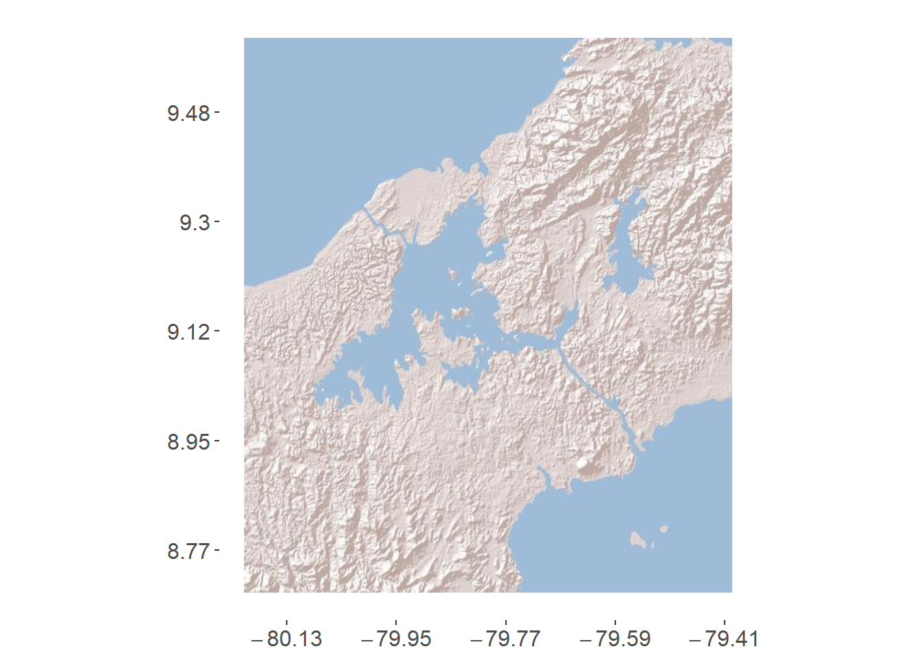

6.3 Figure 2. Climatologies

Total annual precipitation, excluding the lowest correlation CHELSA w5e5

annual_pan<-function(list,extent){
  b<-terra::rast(list)
  c<-terra::app(b,sum)
  d<-terra::crop(c,extent)
  return(d)
}

Stack the climatologies and plot them with the same resolution

# CHELSA 1.2
chelsa_orig<-list.files("../data_reanalysis/CHELSA 1.2/",full.names=TRUE,pattern = ".tif")
chelsa_orig<-annual_pan(chelsa_orig,extentMap)
no_water_mask <- classify(!is.na(chelsa_orig[[1]]), cbind(1, 1), others = NA)
plot(chelsa_orig)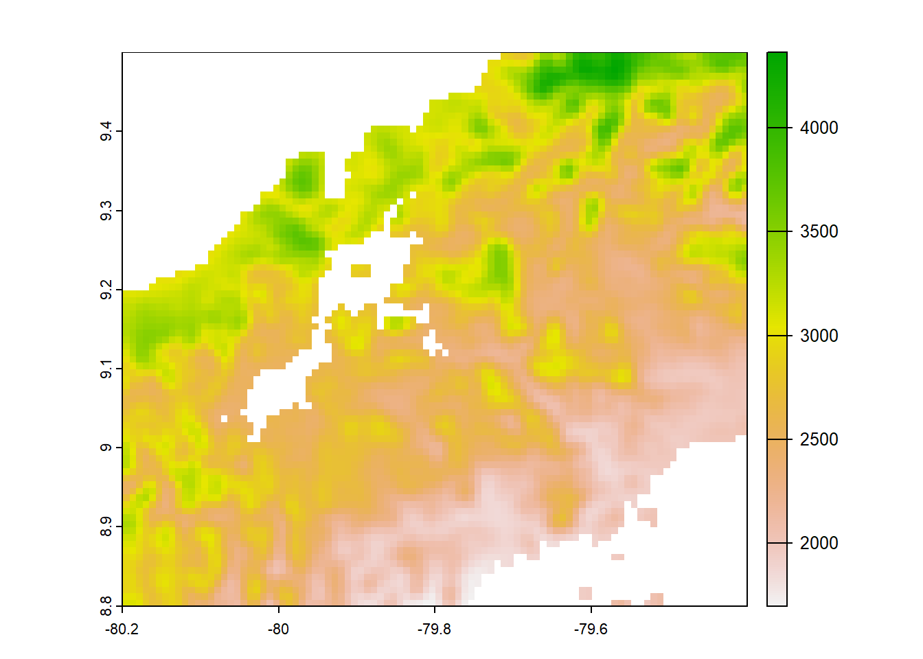

plot(no_water_mask)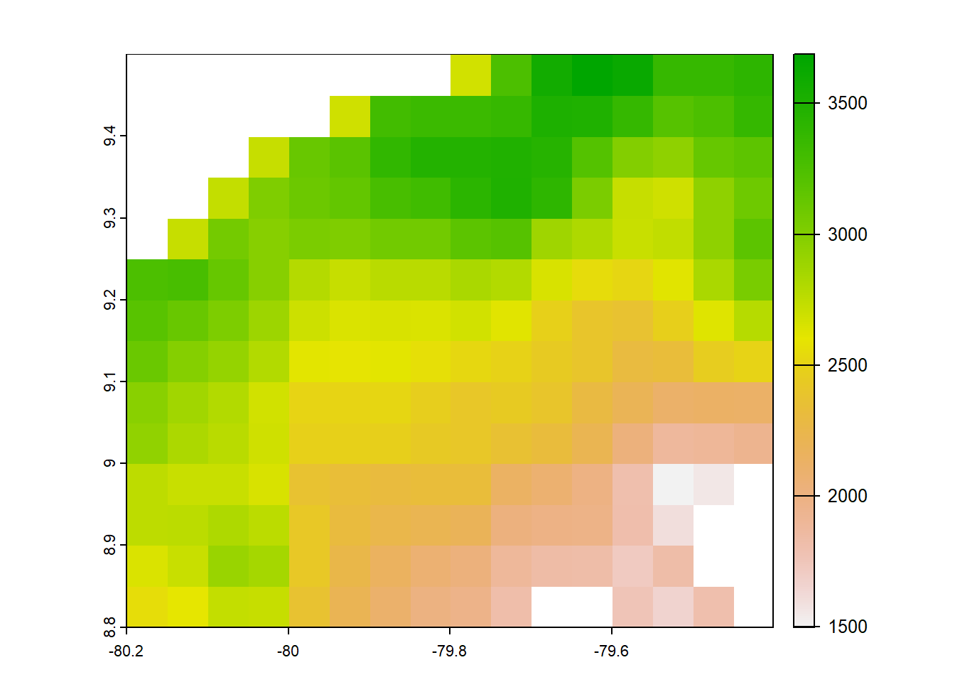

#CHIRPS annual precip at 0.05 
chirps<-list.files("../data_reanalysis/CHIRPS 2.0/climatology",full.name=TRUE,pattern=".tif")
chirps<-annual_pan(chirps,extentMap)
chirps<-terra::project(chirps,chelsa_orig, method='near')
values(chirps)<-ifelse(values(chirps)<0,NA,values(chirps))
plot(chirps)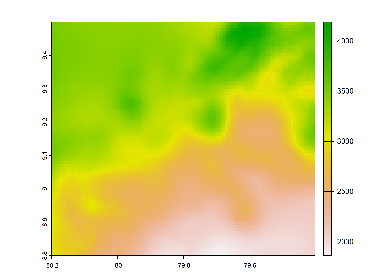

#chelsa 2.1 annual precip 0,0083333 degree orig 
chelsa2_orig<-list.files("../data_reanalysis/CHELSA 2.1",full.names=TRUE,pattern = ".tif")
chelsa2_orig<-annual_pan(chelsa2_orig,extentMap)
crs(chelsa2_orig) <- "EPSG:4326"
chelsa2_orig<- chelsa2_orig*no_water_mask
plot(chelsa2_orig)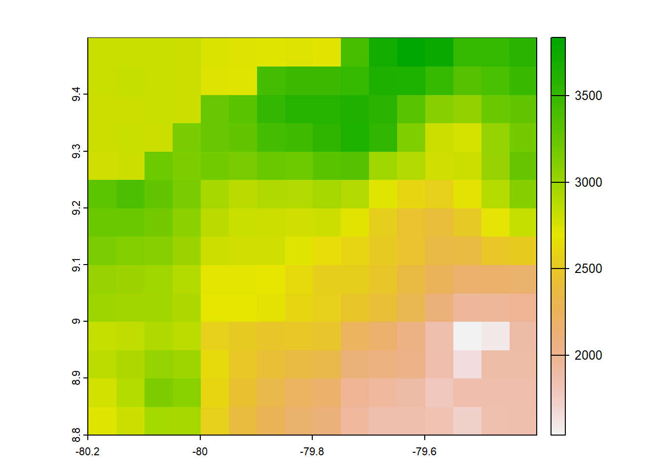

#chp 0.05 degree original 1980-2009 
chp<- list.files("../data_reanalysis/CHPclim",full.names=TRUE,pattern = ".tif")
chp<-annual_pan(chp,extentMap)
chp<-terra::project(chp,chelsa_orig, method='near')
chp<- chp*no_water_mask
plot(chp)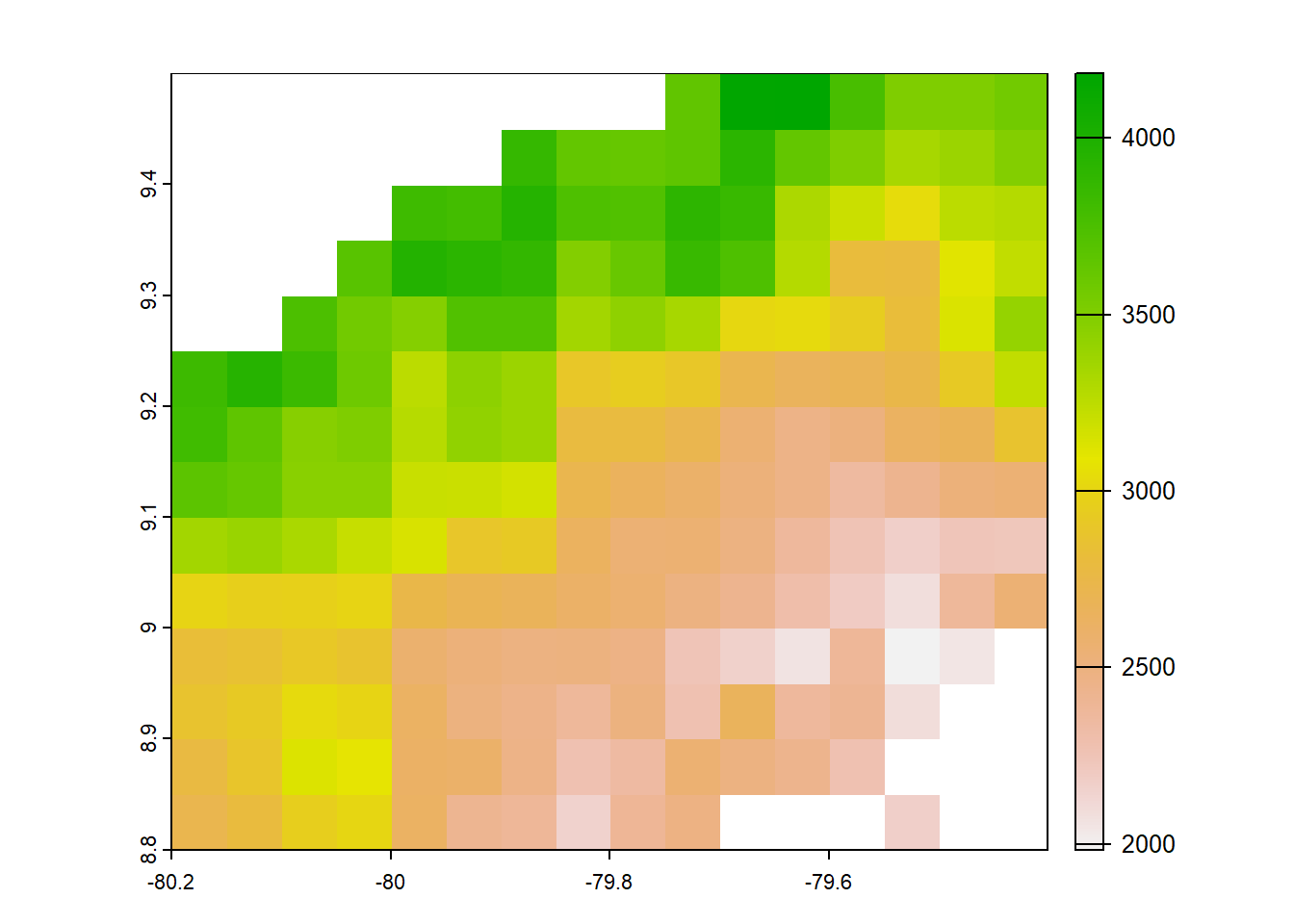

#pbcor 0.05 degree origina
pbcor_chp<- list.files("../data_reanalysis/PBCOR/CHPclim corrected",full.names=TRUE,pattern = ".tif")
pbcor_chp<-annual_pan(pbcor_chp,extentMap)
pbcor_chp<-terra::project(pbcor_chp,chelsa_orig, method='near')
plot(pbcor_chp)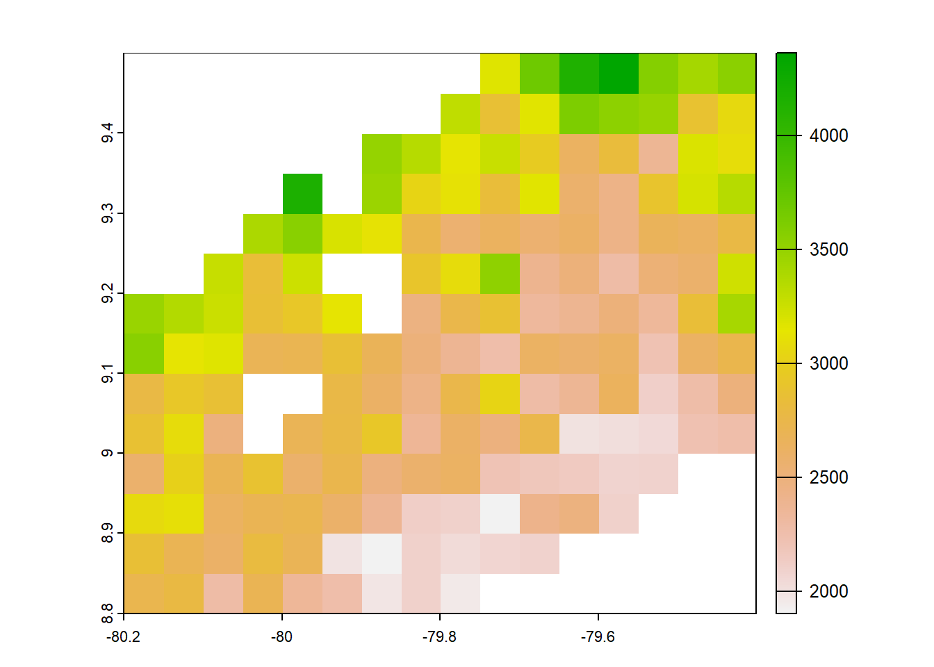

#pbcor 0.05 degree original
pbcor_chelsa<- list.files("../data_reanalysis/PBCOR/CHELSA 1.2 corrected",full.names=TRUE)
pbcor_chelsa<-annual_pan(pbcor_chelsa,extentMap)
pbcor_chelsa<-terra::project(pbcor_chelsa,chelsa_orig,method='near')
plot(pbcor_chelsa)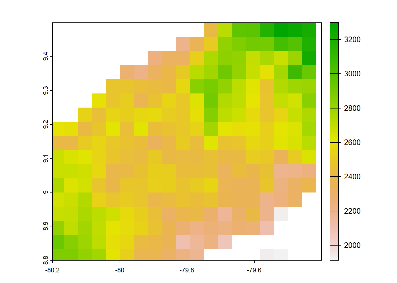

#terra
terra<- list.files("../data_reanalysis/TerraClimate",full.names = TRUE,pattern = "\\.tif$")
terra<-annual_pan(terra,extentMap)
terra<-terra::project(terra,chelsa_orig,method = 'near')
plot(terra)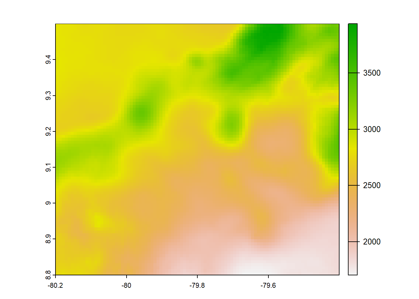

#Chelsa earthenv 2003-2016
chelsaearthenv<-list.files("../data_reanalysis/CHELSA EarthEnv/climatology",full.names = TRUE,pattern = ".tif")
chelsaearthenv<-annual_pan(chelsaearthenv,extentMap)
crs(chelsaearthenv) <- "EPSG:4326"
chelsaearthenv<-chelsaearthenv*no_water_mask
plot(chelsaearthenv)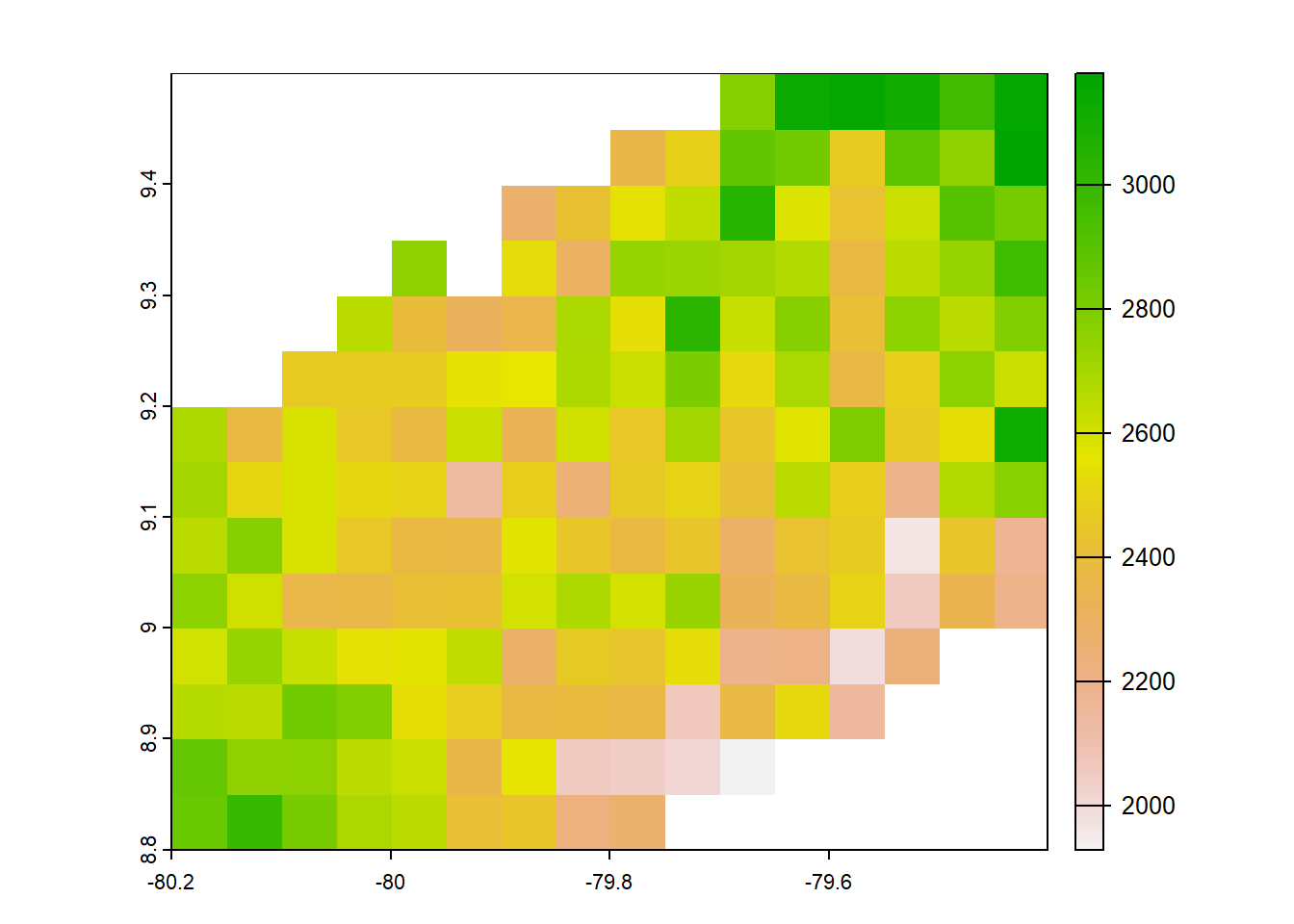

#Pbcorworldclim
pbcor_worldclim<-list.files("../data_reanalysis/PBCOR/WorldClim corrected",full.names = TRUE,pattern = ".tif")
pbcor_worldclim<-annual_pan(pbcor_worldclim,extentMap)
pbcor_worldclim<-terra::project(pbcor_worldclim,chelsa_orig,method="near")
plot(pbcor_worldclim)

#worldclim 
worldclim<-list.files("../data_reanalysis/WorldClim 2.1",full.names=TRUE,pattern=".tif")
worldclim<-annual_pan(worldclim,extentMap)
plot(worldclim)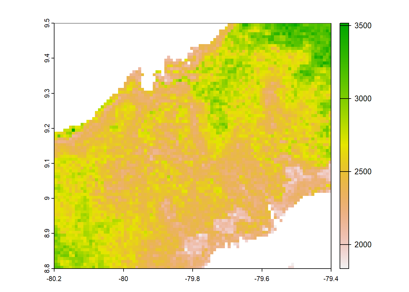

Stack the plots, define a list and plot in a grid

res_stack<-c(chelsa_orig,chelsa2_orig,chelsaearthenv,chirps,chp,terra,worldclim,pbcor_chelsa,pbcor_chp,pbcor_worldclim)

models<-list('layer.1'="CHELSA 1.2",
             'layer.2'="CHELSA 2.1",
             'layer.3'="CHELSA EarthEnv",
             'layer.4'="CHIRPS v2.0",
             'layer.5'="CHPclim v.1.0",
             'layer.6'="TerraClimate",
             'layer.7'="WorldClim v2.1",
             'layer.8'="PBCOR CHELSA 1.2",
             'layer.9'="PBCOR CHPclim",
             'layer.10'="PBCOR WorldClim 2.1"
             )
model2<- function(variable,value){
  return(models[value])
}


jf1<-gplot(res_stack) + 
  geom_raster(aes(fill = value)) +
  facet_wrap(~ variable,labeller=model2,ncol = 5) +
  scale_fill_scico(palette = 'roma',na.value="white",name = "mm/year")+
  coord_equal()+theme_void()+theme(strip.text.x = element_text(size = 8, colour = "black"))+
  labs(title = "Total Annual Precipitation")+ 
  theme(plot.title = element_text(hjust = 0.5,size = 16))

ggsave(path = '../plots',filename = "annual_maps.tiff",  units="in", width=10, height=6, dpi=900)
jf1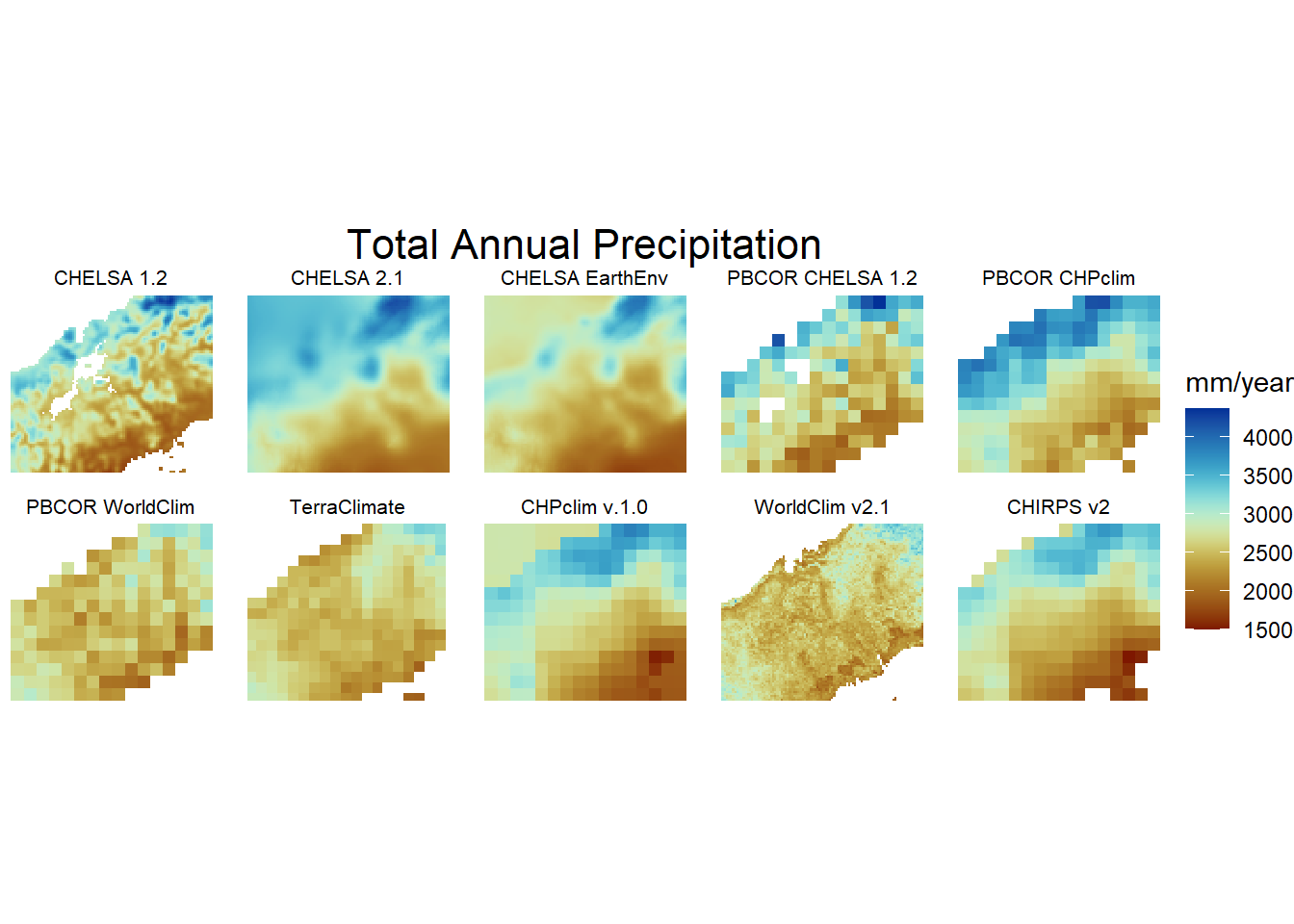

January to April Precipitation individual plots.

# CHELSA 1.2 
chelsa_orig<-list.files("../data_reanalysis/CHELSA 1.2/",full.names=TRUE,pattern = ".tif")
chelsa_orig<-chelsa_orig[1:4]
chelsa_orig<-annual_pan(chelsa_orig,extentMap)
plot(chelsa_orig)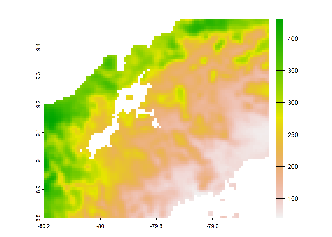

#CHIRPS annual precip at 0.05 
chirps<-list.files("../data_reanalysis/CHIRPS 2.0/climatology",full.name=TRUE,pattern=".tif")
chirps<-chirps[1:4]
chirps<-annual_pan(chirps,extentMap)
chirps<-terra::project(chirps,chelsa_orig, method='near')
values(chirps)<-ifelse(values(chirps)<0,NA,values(chirps))
plot(chirps)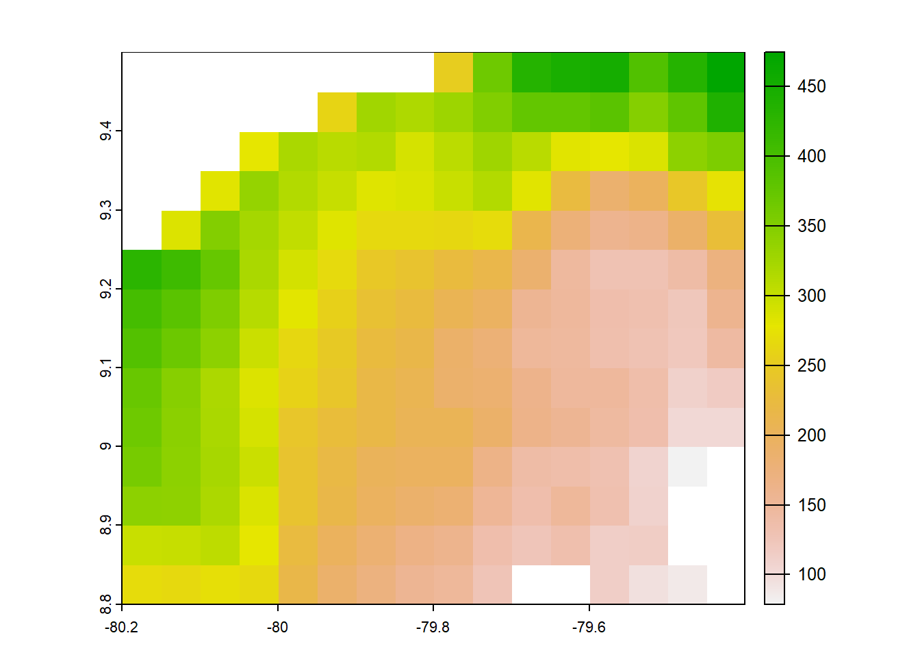

#chelsa 2.1 annual precip 0,0083333 degree orig 
chelsa2_orig<-list.files("../data_reanalysis/CHELSA 2.1",full.names=TRUE,pattern = ".tif")
chelsa2_orig<- chelsa2_orig[1:4]
chelsa2_orig<-annual_pan(chelsa2_orig,extentMap)
crs(chelsa2_orig) <- "EPSG:4326"
chelsa2_orig<- chelsa2_orig*no_water_mask
plot(chelsa2_orig)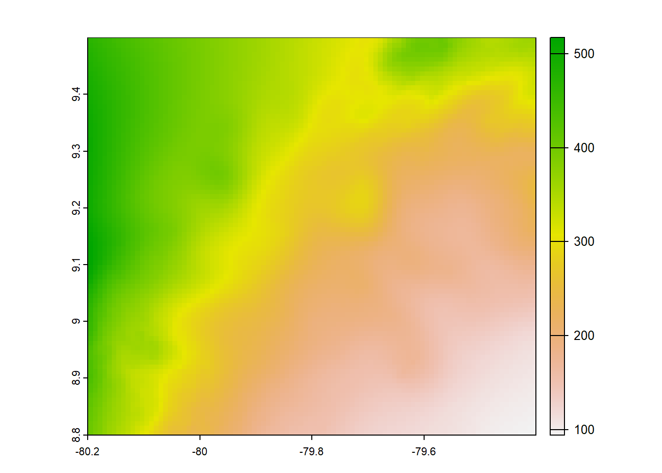

#chp 0.05 degree original 1980-2009 
chp<- list.files("../data_reanalysis/CHPclim",full.names=TRUE,pattern = ".tif")
chp<- chp[1:4]
chp<-annual_pan(chp,extentMap)
chp<-terra::project(chp,chelsa_orig, method='near')
chp<- chp*no_water_mask
plot(chp)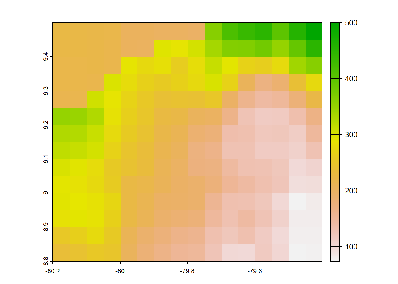

#pbcor 0.05 degree origina
pbcor_chp<- list.files("../data_reanalysis/PBCOR/CHPclim corrected",full.names=TRUE,pattern = ".tif")
pbcor_chp<-pbcor_chp[1:4]
pbcor_chp<-annual_pan(pbcor_chp,extentMap)
pbcor_chp<-terra::project(pbcor_chp,chelsa_orig, method='near')
plot(pbcor_chp)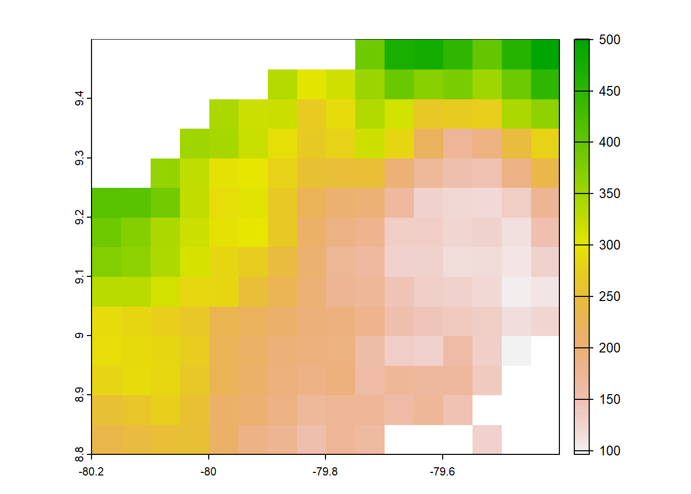

#pbcor 0.05 degree original
pbcor_chelsa<- list.files("../data_reanalysis/PBCOR/CHELSA 1.2 corrected",full.names=TRUE)
pbcor_chelsa<-pbcor_chelsa[1:4]
pbcor_chelsa<-annual_pan(pbcor_chelsa,extentMap)
pbcor_chelsa<-terra::project(pbcor_chelsa,chelsa_orig,method='near')
plot(pbcor_chelsa)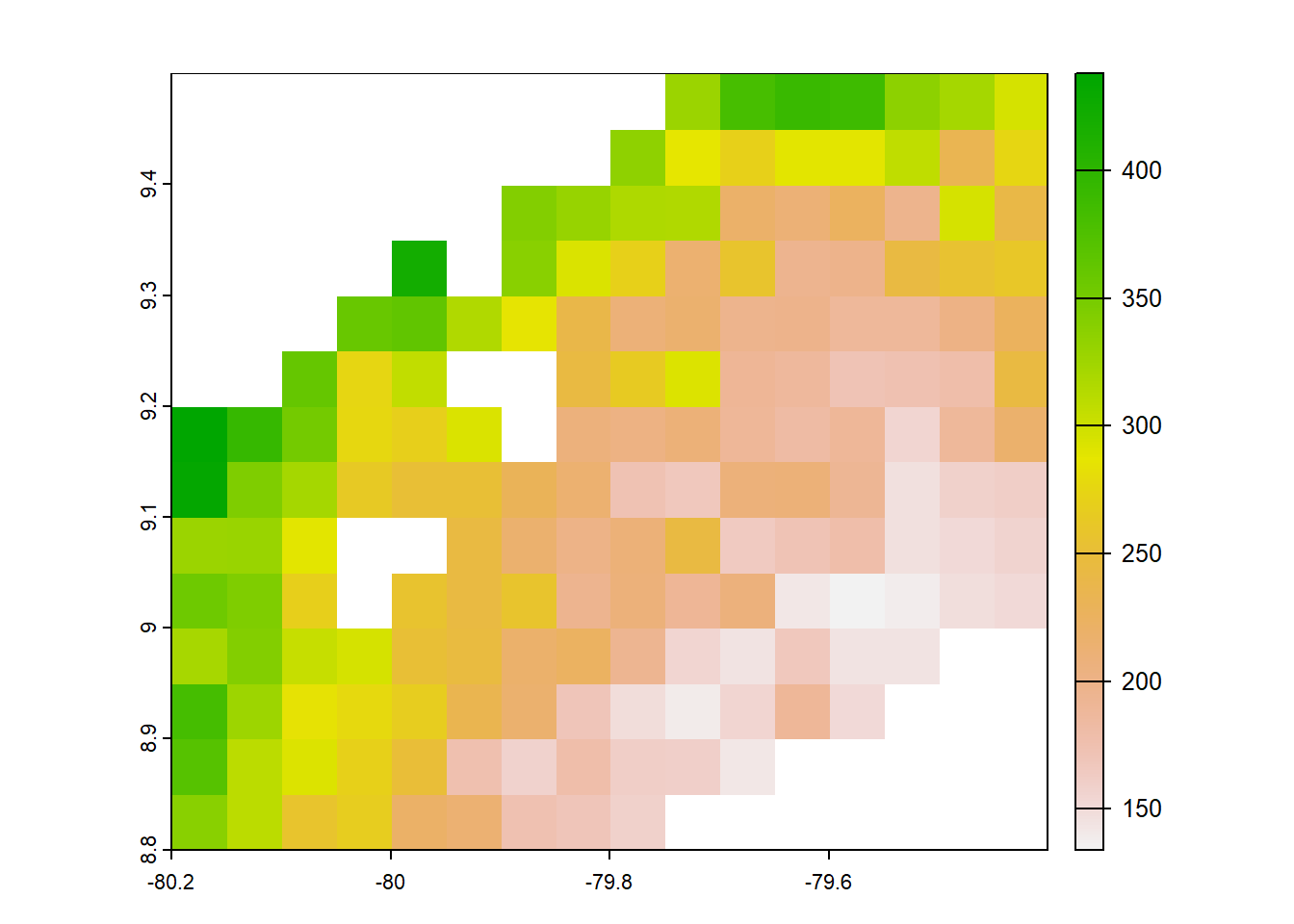

#terra
terra<- list.files("../data_reanalysis/TerraClimate",full.names = TRUE,pattern = "\\.tif$")
terra<-terra[1:4]
terra<-annual_pan(terra,extentMap)
terra<-terra::project(terra,chelsa_orig,method = 'near')
plot(terra)

#Chelsa earthenv 2003-2016
chelsaearthenv<-list.files("../data_reanalysis/CHELSA EarthEnv/climatology",full.names = TRUE,pattern = ".tif")
chelsaearthenv<-chelsaearthenv[1:4]
chelsaearthenv<-annual_pan(chelsaearthenv,extentMap)
crs(chelsaearthenv) <- "EPSG:4326"
chelsaearthenv<-chelsaearthenv*no_water_mask
plot(chelsaearthenv)

#Pbcorworldclim
pbcor_worldclim<-list.files("../data_reanalysis/PBCOR/WorldClim corrected",full.names = TRUE,pattern = ".tif")
pbcor_worldclim<-pbcor_worldclim[1:4]
pbcor_worldclim<-annual_pan(pbcor_worldclim,extentMap)
pbcor_worldclim<-terra::project(pbcor_worldclim,chelsa_orig,method="ngb")

Warning: [project] argument 'method=ngb' is deprecated, it should be
'method=near'

plot(pbcor_worldclim)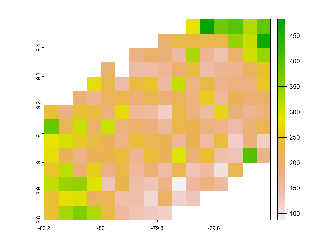

#worldclim 
worldclim<-list.files("../data_reanalysis/WorldClim 2.1",full.names=TRUE,pattern=".tif")
worldclim<-worldclim[1:4]
worldclim<-annual_pan(worldclim,extentMap)
plot(worldclim)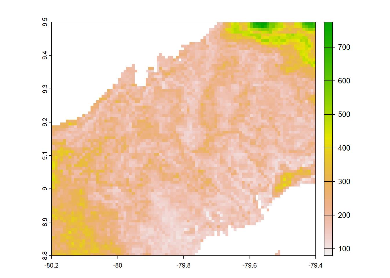

Stack the rasters and plot in a grid.

res_stack_jfma<-c(chelsa_orig,chelsa2_orig,chelsaearthenv,chirps,chp,terra,worldclim,pbcor_chelsa,pbcor_chp,pbcor_worldclim)

models<-list('layer.1'="CHELSA 1.2",
             'layer.2'="CHELSA 2.1",
             'layer.3'="CHELSA EarthEnv",
             'layer.4'="CHIRPS v2.0",
             'layer.5'="CHPclim v.1.0",
             'layer.6'="TerraClimate",
             'layer.7'="WorldClim v2.1",
             'layer.8'="PBCOR CHELSA 1.2",
             'layer.9'="PBCOR CHPclim",
             'layer.10'="PBCOR WorldClim 2.1"
             )
model2<- function(variable,value){
  return(models[value])
}

jf2<-gplot(res_stack_jfma) + 
  geom_raster(aes(fill = value)) +
  facet_wrap(~ variable,labeller=model2,ncol = 5) +
  scale_fill_scico(palette = 'roma',na.value="white",name = "mm")+
  coord_equal()+theme_void()+theme(strip.text.x = element_text(size = 8, colour = "black"))+
  labs(title = "January to April Precipitation")+ 
  theme(plot.title = element_text(hjust = 0.5,size = 16))

ggsave(path = '../plots',filename = "jfma_maps.tiff",  units="in", width=10, height=6, dpi=900)
jf2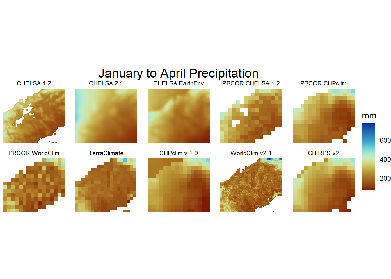

Arrange both combined plots in a grid.

b<-grid.arrange(jf1,jf2,ncol = 1)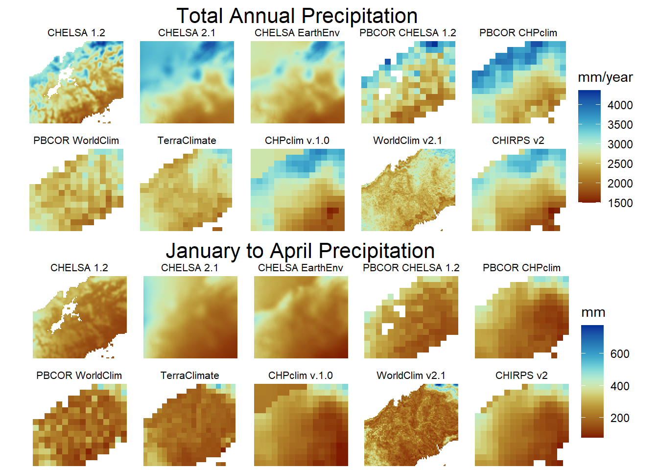

ggsave(b,path='../plots' ,filename = "../plots/climatologies.tiff",  units="in", width=8.25, height=6.25, dpi=900)
b

TableGrob (2 x 1) "arrange": 2 grobs
  z     cells    name           grob
1 1 (1-1,1-1) arrange gtable[layout]
2 2 (2-2,1-1) arrange gtable[layout]

6.4 Figure 3. Annual Bias and January to April Bias

Create data frames for bias of each response variable

precipitation_data_subset <- read.csv(file = "../tables/climatologies.csv")

data_sources <- c("CHELSA.1.2", "CHELSA.2.1", "CHELSA.EarthEnv", "CHIRPS.2.0", 
                  "CHPclim", "TerraClimate", "WorldClim.2.1", "CHELSA.W5E5v1.0",
                  "PBCOR.CHELSA.1.2", "PBCOR.CHPclim", "PBCOR.WorldClim.2.1")

source_names <- c("CHELSA 1.2", "CHELSA 2.1", "CHELSA EarthEnv", "CHPclim", "WorldClim 2.1", "CHIRPS v2.0", 
                  "CHELSA-W5E5v1.0", "TerraClimate", "PBCOR CHELSA 1.2", "PBCOR CHPclim", "PBCOR WorldClim 2.1")


precipitation_data_subset$source <- gsub("CHIRPS 2.0", "CHIRPS v2.0", precipitation_data_subset$source)

bias_frame <- precipitation_data_subset %>% 
  select(site, longitude, latitude, annual, source) %>% 
  mutate(bias = NA)

bias_frame_jfma <- precipitation_data_subset %>% 
  select(site, longitude, latitude, jfma, source) %>% 
  mutate(bias = NA)

for(i in seq_along(data_sources)) {
  bias_frame[bias_frame$source == source_names[i], "bias"] <- 
    precipitation_data_subset[precipitation_data_subset$source == source_names[i], data_sources[i]] - 
    precipitation_data_subset[precipitation_data_subset$source == source_names[i], "annual"]
}

jfma_sources <- paste0(data_sources, "_jfma")
for(i in seq_along(jfma_sources)) {
  bias_frame_jfma[bias_frame_jfma$source == source_names[i], "bias"] <- 
    precipitation_data_subset[precipitation_data_subset$source == source_names[i], jfma_sources[i]] - 
    precipitation_data_subset[precipitation_data_subset$source == source_names[i], "jfma"]
}

bias_frame$source <- factor(bias_frame$source, levels = c("CHELSA 1.2", "CHELSA 2.1", "CHELSA EarthEnv", "CHIRPS v2.0", 
                                                          "CHPclim", "TerraClimate", "WorldClim 2.1", "CHELSA-W5E5v1.0",     
                                                          "PBCOR CHELSA 1.2", "PBCOR CHPclim", "PBCOR WorldClim 2.1"))

bias_frame_jfma$source <- factor(bias_frame_jfma$source, levels = c("CHELSA 1.2", "CHELSA 2.1", "CHELSA EarthEnv", "CHIRPS v2.0", 
                                                                    "CHPclim", "TerraClimate", "WorldClim 2.1", "CHELSA-W5E5v1.0",     
                                                                    "PBCOR CHELSA 1.2", "PBCOR CHPclim", "PBCOR WorldClim 2.1"))

Convert to other coordinate system for plotting purposes

bias_frame <- bias_frame %>%
  st_as_sf(coords = c("longitude","latitude"), crs = 4326) %>%
  st_transform(3857) %>%
  cbind(st_coordinates(.)) %>%
  rename(longitude_3857 = X, latitude_3857 = Y)%>%
  filter(source!="CHELSA-W5E5v1.0")

bias_frame_jfma <- bias_frame_jfma %>%
  st_as_sf(coords = c("longitude","latitude"), crs = 4326) %>%
  st_transform(3857) %>%
  cbind(st_coordinates(.)) %>%
  rename(longitude_3857 = X, latitude_3857 = Y)%>%
  filter(source!="CHELSA-W5E5v1.0")

Plot the panels for each response variable.

max_abs_bias <- max(abs(bias_frame$bias), na.rm = TRUE)
Bias_annual_panels <- basemap_ggplot(bbox_sf, map_service = "esri", map_type = "world_shaded_relief", map_res= 2) +
  theme_void() +
  geom_jitter(data = bias_frame,
              aes(x = longitude_3857, y = latitude_3857, colour = bias),
              size = 2, width = 0.3, height = 0.3) +
  geom_jitter(data = bias_frame,
              aes(x = longitude_3857, y = latitude_3857),
              size = 2, shape = 21, width = 0.3, height = 0.3) +
  scale_color_scico(palette = "roma", direction = -1, 
                    midpoint = 0, 
                    limits = c(-max_abs_bias, max_abs_bias))+
  facet_wrap(~source,ncol=5) +
  coord_equal()+
  labs(color = "Bias (mm)") +
  ggtitle("Total Annual Precipitation")+ theme(legend.title = element_text(size = 10))

Loading basemap 'world_shaded_relief' from map service 'esri'...
Using geom_raster() with maxpixels = 1202280.

max_abs_bias_jfma <- max(abs(bias_frame_jfma$bias), na.rm = TRUE)

Bias_jfma_panels <- basemap_ggplot(bbox_sf, map_service = "esri", map_type = "world_shaded_relief", map_res= 2) +
  theme_void() +
  geom_jitter(data = bias_frame_jfma,
              aes(x = longitude_3857, y = latitude_3857, colour = bias),
              size = 2, width = 0.3, height = 0.3) +
  geom_jitter(data = bias_frame_jfma,
              aes(x = longitude_3857, y = latitude_3857),
              size = 2, shape = 21, width = 0.3, height = 0.3) +
  scale_color_scico(palette = "roma", direction = -1, 
                    midpoint = 0, 
                    limits = c(-max_abs_bias_jfma, max_abs_bias_jfma)) +
  facet_wrap(~source,ncol = 5) +
  coord_equal()+
  labs(color = "Bias (mm)") +
  ggtitle("January to April Precipitation") + theme(legend.title = element_text(size = 10))

Loading basemap 'world_shaded_relief' from map service 'esri'...
Using geom_raster() with maxpixels = 1202280.

Bias_annual_panels <- Bias_annual_panels +
  theme(strip.text = element_text(size = 7),
        plot.title = element_text(hjust = 0.5,size=14),
        plot.background = element_rect(fill = "white"))

Bias_jfma_panels <- Bias_jfma_panels +
  theme(strip.text = element_text(size = 7),
        plot.title = element_text(hjust = 0.5,size=14),
        plot.background = element_rect(fill = "white"))

#ggsave(Bias_annual_panels,path = '../plots',filename = "annual_bias_maps.tiff",  units="in", width=10, height=10, dpi=900)
#ggsave(Bias_jfma_panels,path = '../plots',filename = "jfma_bias_maps.tiff",  units="in", width=10, height=10, dpi=900)
#Bias_annual_panels
#Bias_jfma_panels

Arrange both set of panels in a grid

c<-grid.arrange(Bias_annual_panels,Bias_jfma_panels,ncol = 1)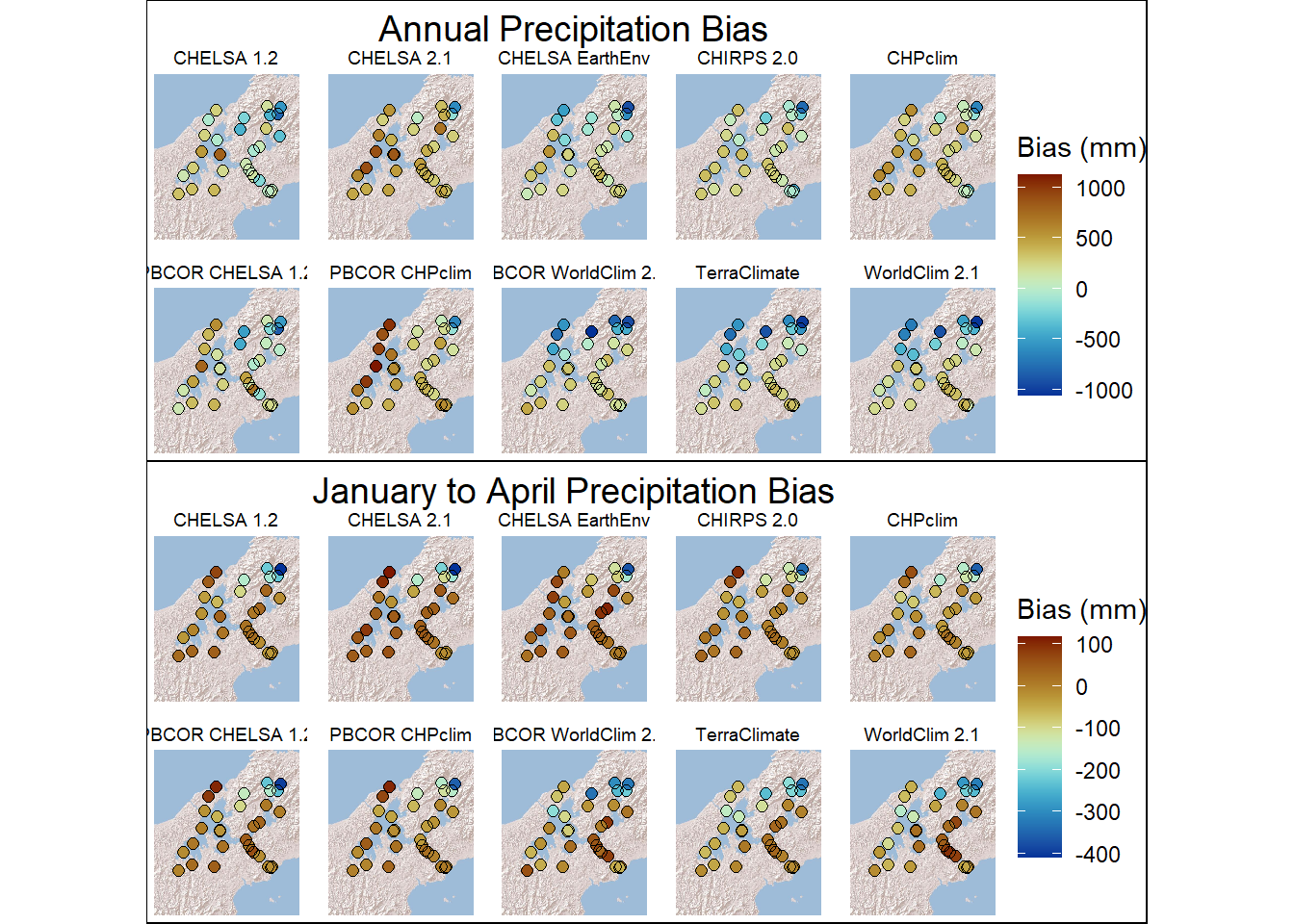

ggsave(c,path='../plots' ,filename = "../plots/bias_figure.tiff",  units="in", width=9, height=6, dpi=900)
c

TableGrob (2 x 1) "arrange": 2 grobs
  z     cells    name           grob
1 1 (1-1,1-1) arrange gtable[layout]
2 2 (2-2,1-1) arrange gtable[layout]

6.5 Figure 4. Correlation plots

precipitation_data_subset <- read.csv(file="../tables/climatologies.csv")

source_names <- c("CHELSA 1.2", "CHELSA 2.1", "CHELSA EarthEnv", "CHPclim", "WorldClim 2.1", "CHIRPS v2.0", 
                  "CHELSA-W5E5v1.0", "TerraClimate", "PBCOR CHELSA 1.2", "PBCOR CHPclim", "PBCOR WorldClim 2.1")

precipitation_data_subset$source <- gsub("CHIRPS 2.0", "CHIRPS v2.0", precipitation_data_subset$source)

corr_frame <- precipitation_data_subset %>% 
  select("site","longitude","latitude","annual","source") %>% 
  mutate(value=NA)
corr_frame_jfma<- precipitation_data_subset %>% 
  select("site","longitude","latitude","jfma","source") %>% 
  mutate(value=NA)

for(i in seq_along(data_sources)) {
  corr_frame[corr_frame$source == source_names[i], "value"] <- precipitation_data_subset[precipitation_data_subset$source == source_names[i], data_sources[i]]
}
jfma_sources <- paste0(data_sources, "_jfma")
for(i in seq_along(jfma_sources)) {
  corr_frame_jfma[corr_frame_jfma$source == source_names[i], "value"] <- precipitation_data_subset[precipitation_data_subset$source == source_names[i], jfma_sources[i]] 
}
corr_frame$source <- factor(corr_frame$source, levels = c("CHELSA 1.2","CHELSA 2.1","CHELSA EarthEnv", "CHIRPS v2.0","CHPclim",            
                                                                            "TerraClimate","WorldClim 2.1","CHELSA-W5E5v1.0",     
                                                                            "PBCOR CHELSA 1.2","PBCOR CHPclim","PBCOR WorldClim 2.1"))
corr_frame_jfma$source <- factor(corr_frame_jfma$source, levels = c("CHELSA 1.2","CHELSA 2.1","CHELSA EarthEnv", "CHIRPS v2.0","CHPclim",  
                                                                            "TerraClimate","WorldClim 2.1","CHELSA-W5E5v1.0",     
                                                                            "PBCOR CHELSA 1.2","PBCOR CHPclim","PBCOR WorldClim 2.1"))

Plot using ggplot

annual_corr<-ggplot(corr_frame[corr_frame$source!="CHELSA-W5E5v1.0",],aes(x = value,y=annual))+
  geom_smooth(method='lm',se=FALSE)+geom_abline(slope = 1, intercept = 0, lty= 2)+
  geom_point(col=rgb(0,0,0,alpha=0.5))+facet_wrap(vars(source),ncol=5)+
  theme_classic()+
  expand_limits(x=c(1000,4500),y=c(1000,4500))+
  coord_equal()+
  theme(
    strip.text = element_text(size = 8)  
  )

dat_text <- data.frame(
  source  = unique(corr_frame[corr_frame$source!="CHELSA-W5E5v1.0","source"])
)

for(i in 1:10){
  model <- lm(value ~ annual, data = corr_frame[corr_frame$source == dat_text$source[i],])
  dat_text$eq[i] <- paste0("y = ", round(coef(model)[1], 2), " + ", round(coef(model)[2], 2), "x")
}
annual_corr<-annual_corr + geom_text(
  data    = dat_text,
  mapping = aes(x = 1800, y = 1300, label = eq),
  hjust   = 0,
  vjust   = 1,
  size    = 2
)+labs(title = "Total Annual Precipitation")+ 
  xlab("Gridded products annual precipitation (mm)") +
  ylab("In-situ annual precipitation (mm)") 

ggsave(annual_corr,path='../plots' ,filename = "../plots/correlation_annual.tiff",  units="in", width=8.25, height=7.25, dpi=900)

`geom_smooth()` using formula = 'y ~ x'

annual_corr

`geom_smooth()` using formula = 'y ~ x'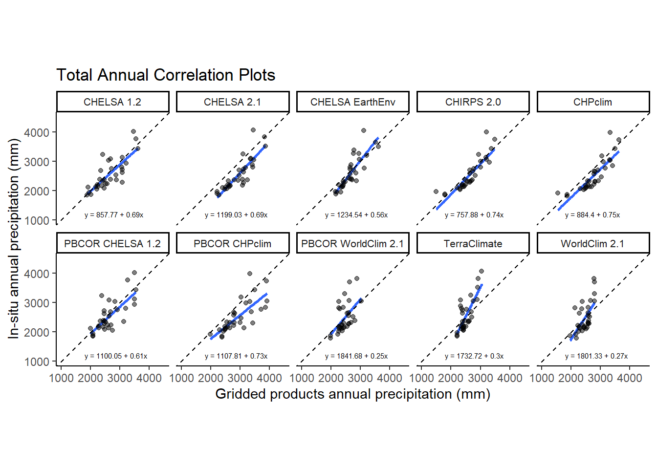

Plot January to April correlation plots

jfma_corr<-ggplot(corr_frame_jfma[corr_frame_jfma$source!="CHELSA-W5E5v1.0",],aes(x = value,y=jfma))+
  geom_smooth(method='lm',se=FALSE)+geom_abline(slope = 1, intercept = 0, lty= 2)+
  geom_point(col=rgb(0,0,0,alpha=0.5))+facet_wrap(vars(source),ncol=5)+
  expand_limits(x=c(0,800),y=c(0,800))+
  theme_classic()+
  coord_equal()+
  theme(
    strip.text = element_text(size = 8)  
  )

dat_text <- data.frame(
  source  = unique(corr_frame_jfma[corr_frame_jfma$source!="CHELSA-W5E5v1.0","source"])
)

for(i in 1:10){
  model <- lm(value ~ jfma, data = corr_frame_jfma[corr_frame_jfma$source == dat_text$source[i],])
  dat_text$eq[i] <- paste0("y = ", round(coef(model)[1], 2), " + ", round(coef(model)[2], 2), "x")
}
jfma_corr<-jfma_corr + geom_text(
  data    = dat_text,
  mapping = aes(x = 350, y = 50, label = eq),
  hjust   = 0,
  vjust   = 1,
  size    = 2
)+labs(title = "January to April Precipitation")+ 
  xlab("Gridded products Jan-Apr precipitation (mm)") +
  ylab("In-situ Jan-Apr precipitation (mm)") 

ggsave(jfma_corr,path='../plots' ,filename = "../plots/correlation_jfma.tiff",  units="in", width=8, height=7, dpi=900)

`geom_smooth()` using formula = 'y ~ x'

jfma_corr

`geom_smooth()` using formula = 'y ~ x'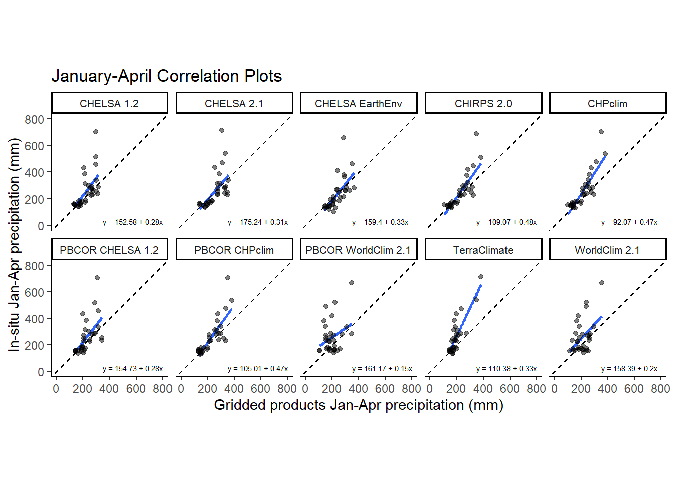

Arrange both correlation panels in a grid

d<-grid.arrange(annual_corr,jfma_corr,ncol = 1)

`geom_smooth()` using formula = 'y ~ x'
`geom_smooth()` using formula = 'y ~ x'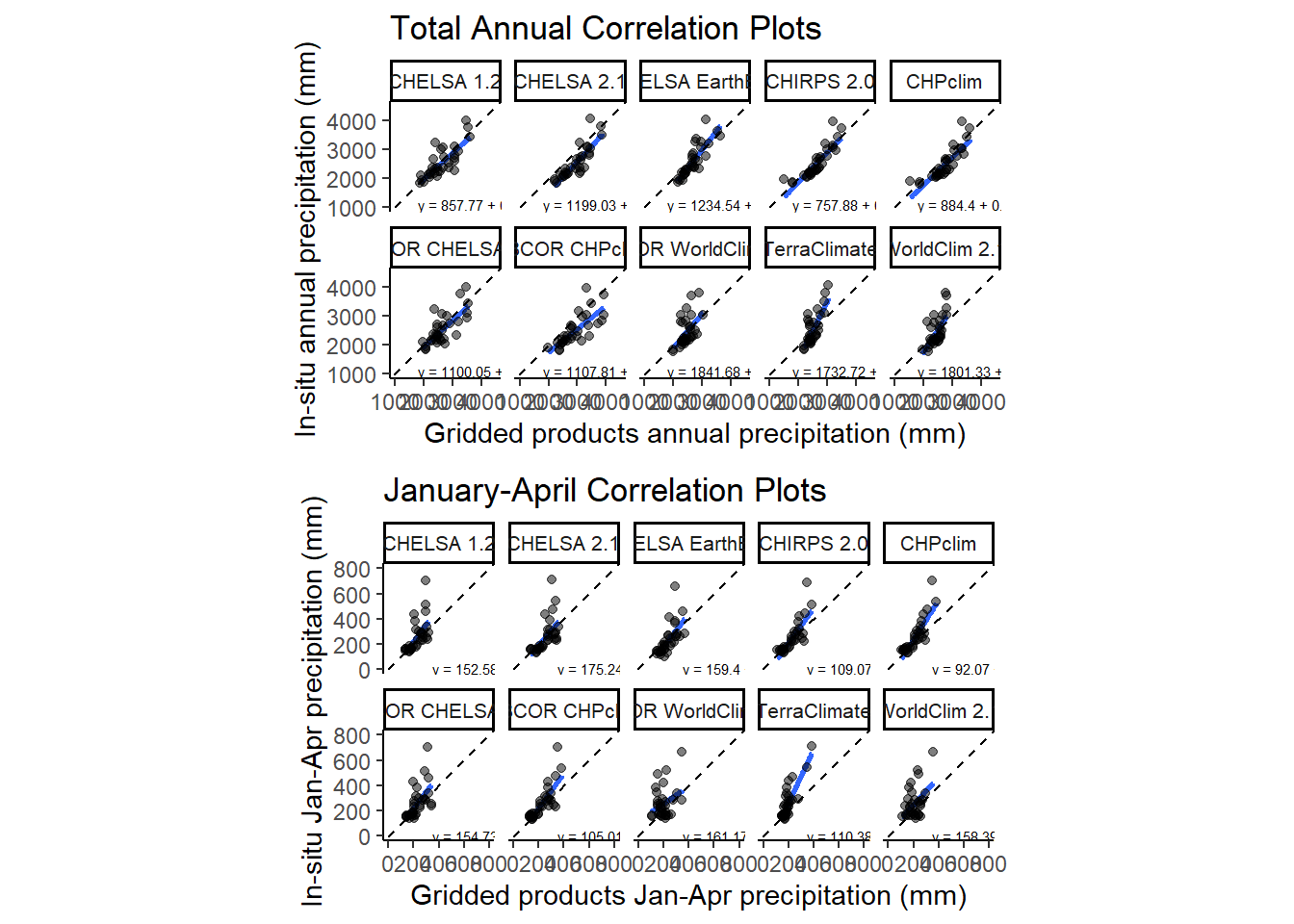

ggsave(d,path='../plots' ,filename = "../plots/correlation.tiff",  units="in", width=7.5, height=7.5, dpi=900)

6.6 Figure.5 Seasonality plots

Mutating the data is necessary to consider a second line representing a second set of ground data in BCI.

acp38_ag <- read.csv("../tables/acp38_ag.csv")

acp38_ag$dataset_name <- gsub("CHIRPS 2.0", "CHIRPS v2.0", acp38_ag$dataset_name)

acp38_ag_long <- acp38_ag %>%
  tidyr::pivot_longer(
    cols = c(CHELSA1.2, CHELSA2.1, CHELSA_EarthEnv, CHELSAW5E5v1.0,
             CHIRPS2.0, CHPclim, TerraClimate, WorldClim2.1,
             PBCOR_CHELSA1.2, PBCOR_CHPclim, PBCOR_WorldClim2.1),
    names_to = "colname",
    values_to = "value"
  ) %>%
  mutate(colname = case_when(
    colname == "CHELSA1.2" ~ "CHELSA 1.2",
    colname == "CHELSA2.1" ~ "CHELSA 2.1",
    colname == "CHELSA_EarthEnv" ~ "CHELSA EarthEnv",
    colname == "CHPclim" ~ "CHPclim",
    colname == "WorldClim2.1" ~ "WorldClim 2.1",
    colname == "CHIRPS2.0" ~ "CHIRPS v2.0",  # Match this AFTER pivot
    colname == "CHELSAW5E5v1.0" ~ "CHELSA-W5E5v1.0",
    colname == "TerraClimate" ~ "TerraClimate",
    colname == "PBCOR_CHELSA1.2" ~ "PBCOR CHELSA 1.2",
    colname == "PBCOR_CHPclim" ~ "PBCOR CHPclim",
    colname == "PBCOR_WorldClim2.1" ~ "PBCOR WorldClim 2.1"
  )) %>%
  filter((dataset_name == colname) | (dataset_name == "Ground" & colname == "CHELSA 1.2")) %>%
  mutate(value = ifelse(dataset_name == "Ground", mon_mean, value)) %>%
  mutate(dataset_name = ifelse(site == "BCICLEAR" & dataset_name == "Ground", "Ground manual", dataset_name)) %>%
  filter(!(site == "BCICLEAR" & dataset_name != "Ground manual")) %>%
  mutate(site = ifelse(site == "BCICLEAR", "BCI", site))


year<- acp38_ag_long %>% filter(dataset_name=="Ground")%>%
  group_by(site) %>% summarise(annual_mean=sum(value,na.rm=TRUE))

acp38_ag_long$dataset_name <- factor(acp38_ag_long$dataset_name, levels = c("CHELSA 1.2","CHELSA 2.1","CHELSA EarthEnv","CHELSA-W5E5v1.0",
                                                                            "CHIRPS v2.0","CHPclim", "TerraClimate","WorldClim 2.1",             
                                                                            "PBCOR CHELSA 1.2","PBCOR CHPclim","PBCOR WorldClim 2.1","Ground",  
                                                                             "Ground manual"))
unique(acp38_ag_long$dataset_name)

 [1] CHELSA 1.2          CHELSA 2.1          CHELSA EarthEnv    
 [4] CHPclim             WorldClim 2.1       CHIRPS v2.0        
 [7] CHELSA-W5E5v1.0     TerraClimate        PBCOR CHELSA 1.2   
[10] PBCOR CHPclim       PBCOR WorldClim 2.1 Ground             
[13] Ground manual      
13 Levels: CHELSA 1.2 CHELSA 2.1 CHELSA EarthEnv ... Ground manual

site_labels <- setNames(
  paste0(
    year$site, " (", round(year$annual_mean, 0), " mm/yr)"
  ),
  year$site
)

acp38_ag_long$site <- factor(acp38_ag_long$site,    # Reordering group factor levels
                               levels = c("SANMIGUEL", "AGUACLARA", "PELUCA", "BCI","GUACHA","CASCADAS","GAMBOA","PEDROMIGUEL"))

Plot using ggplot2 and customs colors

seasonality_plot <- ggplot(acp38_ag_long, aes(x = Month, y = value)) +
  geom_line(aes(color = dataset_name, linewidth = dataset_name)) +
  geom_point(aes(color = dataset_name), size = 0.2) +
  facet_wrap(
    vars(site),
    ncol = 4,
    labeller = labeller(site = site_labels)
  ) +
  scale_color_manual(
    labels = c(
      "CHELSA 1.2", "CHELSA 2.1", "CHELSA EarthEnv", "CHELSA-W5E5v1.0",
      "CHIRPS v2.0", "CHPclim", "TerraClimate", "WorldClim 2.1",
      "PBCOR CHELSA 1.2", "PBCOR CHPclim", "PBCOR WorldClim 2.1",
      "Ground", "Ground manual"
    ),
    values = c(
      '#1f78b4', '#b2df8a', '#33a02c', '#fb9a99', '#e31a1c', '#fdbf6f',
      '#ff7f00', '#cab2d6', '#6a3d9a', '#a6cee3', 'brown', "black", "purple"
    )
  ) +
  scale_discrete_manual(
    "linewidth",
    values = c(0.2, 0.2, 0.2, 0.2, 0.2, 0.2, 0.2, 0.2, 0.2, 0.2, 0.2, 0.5, 0.5)
  ) +
  scale_x_continuous(
    breaks = 1:12,
    labels = c("Jan", "Feb", "Mar", "Apr", "May", "Jun",
               "Jul", "Aug", "Sep", "Oct", "Nov", "Dec")
  ) +
  theme_classic() +
  theme(
    axis.text.x = element_text(angle = 60, vjust = 1.2, hjust = 1, size = 7),
    strip.text = element_text(size = 6),
    axis.text.y = element_text(size = 7),
    axis.title.x = element_text(size = 8),
    axis.title.y = element_text(size = 8),
    legend.text = element_text(size = 7),
    legend.title = element_text(size = 8)
  ) +
  ylab("Monthly Precipitation (mm)") +
  labs(
    color = "Gridded dataset"
  ) +
  guides(linewidth = "none")

ggsave(seasonality_plot,path='../plots' ,filename = "../plots/seasonality.tiff",  units="in", width=7.25, height=5, dpi=900)
seasonality_plot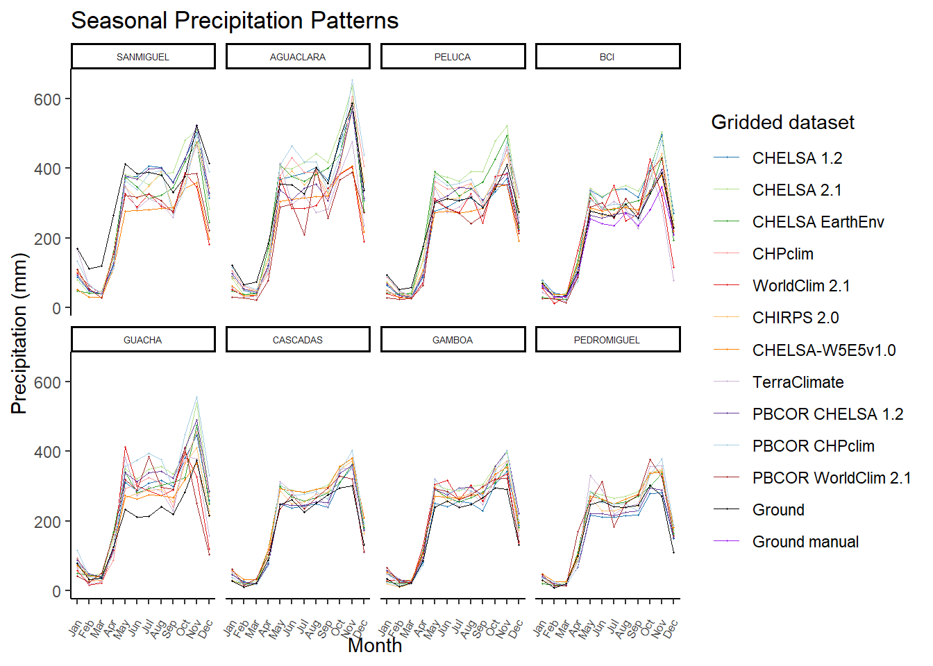

6.7 Figure 6. Interannual variability

Mutating the dataset to consider the existence of a second line representing another set of ground data coming from a secondary rain gauge in BCI.

acp38_year<-read.csv("../tables/acp38_year.csv")
acp38_year$dataset_name <- gsub("CHIRPS 2.0", "CHIRPS v2.0", acp38_year$dataset_name)

acp38_year_long<- acp38_year%>%
  tidyr::pivot_longer(cols=c(annual_precip,CHELSA1.2:TerraClimate), names_to = "colname", values_to = "value")%>%
  mutate(colname = case_when(
    colname == "CHELSA1.2" ~ "CHELSA 1.2",
    colname == "CHELSA2.1" ~ "CHELSA 2.1",
    colname == "CHELSA_EarthEnv" ~ "CHELSA EarthEnv",
    colname == "CHIRPS2.0" ~ "CHIRPS v2.0",
    colname == "CHELSAW5E5v1.0" ~ "CHELSA-W5E5v1.0",
    colname == "TerraClimate" ~ "TerraClimate",
    colname == "annual_precip" ~ "Ground"
  ))%>%
  filter((dataset_name == colname) | (dataset_name == "CHELSA 1.2" & colname == "Ground"))%>%
  mutate(dataset_name= ifelse(dataset_name == "CHELSA 1.2" & colname == "Ground"& site=="BCICLEAR","Ground manual",dataset_name))%>%
  filter(!(site == "BCICLEAR" & dataset_name != "Ground manual"))%>%
  mutate(site=ifelse(site=="BCICLEAR","BCI",site))%>%
  mutate(dataset_name=ifelse(dataset_name=="CHELSA 1.2"&colname=="Ground","Ground",dataset_name))

year<- acp38_year_long %>% filter(dataset_name=="Ground")%>%
  group_by(site) %>% summarise(annual_mean=mean(value,na.rm=TRUE))

acp38_year_long$site <- factor(acp38_year_long$site,      # Reordering group factor levels
                    levels = c("SANMIGUEL", "AGUACLARA", "PELUCA", "BCI","GUACHA","CASCADAS","GAMBOA","PEDROMIGUEL"))

site_labels <- setNames(
  paste0(
    year$site, " (", round(year$annual_mean, 0), " mm/yr)"
  ),
  year$site
)
acp38_year_long$dataset_name<-factor(acp38_year_long$dataset_name,
                                     levels=c("CHELSA 1.2","CHELSA 2.1", "CHELSA EarthEnv","CHELSA-W5E5v1.0","CHIRPS v2.0","TerraClimate","Ground","Ground manual"))
acp38_year_long <- acp38_year_long %>%
  filter(!is.na(dataset_name))

Plot using ggplot2

interannual_plot <- ggplot(acp38_year_long, aes(x = Year, y = value)) +
  geom_line(aes(color = dataset_name, linewidth= dataset_name))+
  geom_point(aes(color = dataset_name), size = 0.2) +
  expand_limits(x = c(1970, 2016), y = c(900, 5900)) +
  facet_wrap(vars(site), ncol = 4, labeller = labeller(site = site_labels)) +
  theme_classic() +
  xlab("Year") +
  ylab("Annual Precipitation (mm)") +
  labs(color = "Gridded dataset") +
  theme(
    strip.text = element_text(size = 7),
    axis.text.x = element_text(size = 7),
    axis.text.y = element_text(size = 7),
    axis.title.x = element_text(size = 8),
    axis.title.y = element_text(size = 8),
    legend.text = element_text(size = 7),
    legend.title = element_text(size = 8)
  ) +
  scale_color_manual(values = c(
    "CHELSA 1.2" = "#a65628",
    "CHELSA 2.1" = "#e7298a",
    "CHELSA EarthEnv" = "#e31a1c",
    "CHIRPS v2.0" = "#ff7f00",
    "CHELSA-W5E5v1.0" = "#984ea3",
    "TerraClimate" = "#4daf4a",
    "Ground" = "black",
    "Ground manual" = "purple"
  )) +
  scale_discrete_manual("linewidth",values = c(0.2, 0.2, 0.2, 0.2, 0.2, 0.2, 0.5, 0.5))+
  guides(linewidth = "none")


##annual
ggsave(interannual_plot,path='../plots' ,filename = "../plots/interannual.tiff",  units="in", width=8.25, height=4, dpi=900)

Warning: Removed 77 rows containing missing values or values outside the scale range
(`geom_line()`).

Warning: Removed 618 rows containing missing values or values outside the scale range
(`geom_point()`).

interannual_plot

Warning: Removed 77 rows containing missing values or values outside the scale range
(`geom_line()`).
Removed 618 rows containing missing values or values outside the scale range
(`geom_point()`).

Auguie, Baptiste, and Anton Antonov. 2017. gridExtra: Miscellaneous Functions for "Grid" Graphics. https://doi.org/10.32614/CRAN.package.gridExtra.

Crameri, Fabio. 2023. “Scientific Colour Maps.” Zenodo. https://doi.org/10.5281/ZENODO.1243862.

Oscar Perpiñán, and Robert Hijmans. 2023. rasterVis. https://oscarperpinan.github.io/rastervis/.

Pebesma, Edzer. 2018. “Simple Features for R: Standardized Support for Spatial Vector Data.” The R Journal 10 (1): 439–46. https://doi.org/10.32614/RJ-2018-009.

Schwalb-Willmann, Jakob. 2024. Basemaps: Accessing Spatial Basemaps in r.