3  Ground data wrangling and cleaning

3.1 About

We use the term “ground data” to refer to rain gauge observations collected from meteorological stations managed by the Smithsonian Tropical Research Institute and the Panama Canal Authority (Autoridad del Canal de Panamá). First, we merged both datasets and addressed key questions to establish criteria for selecting the stations to be included in the analysis. We then calculated annual precipitation and January-to-April precipitation, the latter serving as a proxy for dry season precipitation. Data visualization was used to identify the sites that meet the minimum criteria. We used the lmer4 package to fit a linear mixed model, using year as a random effect and site as a fixed effect across the full time period. The time series was filtered for the 1970-2016 period, ensuring no site was duplicated. We retained all actual values and gap-filled missing data using the predicted values from the model.

3.2 Libraries

library(dplyr)
library(tidyr)
library(ggplot2)
library(lme4)

3.3 The data

The github repository contains a version of the data that has been cleaned and calculated into monthly values.Data provided by the Meteorological and Hydrological Branch of the Panama Canal Authority and the Physical Monitoring Program of the Smithsonian Tropical Research Institute.

ACP_DATA<- "../data_ground/met_data/ACP_data/cleanedVV/ACP_data.csv"
STRI_DATA<-"../data_ground/met_data/STRI_data/STRI_monthlyPrecip.csv"

We read in the data using base R function read.csv()

acpDATA<- read.csv(ACP_DATA)
striDATA<- read.csv(STRI_DATA)

First we bind the rows of both data sources and create year and month columns

monthlyPrecipData<- acpDATA%>%bind_rows(striDATA)
monthlyPrecipData$year<- as.numeric(format(as.Date(monthlyPrecipData$month_year, format="%Y-%m-%d"),"%Y"))
monthlyPrecipData$month<- as.numeric(format(as.Date(monthlyPrecipData$month_year, format="%Y-%m-%d"),"%m"))

How many stations there is in each of the years?

nstations<- monthlyPrecipData %>% group_by(year)%>% filter(!is.na(monthly_precip))%>%summarize(nstations= n_distinct(site))

ggplot(nstations, aes(x=year,y=nstations))+
  geom_point()+
  theme_bw()+
  labs(x="Year", y="Number of stations")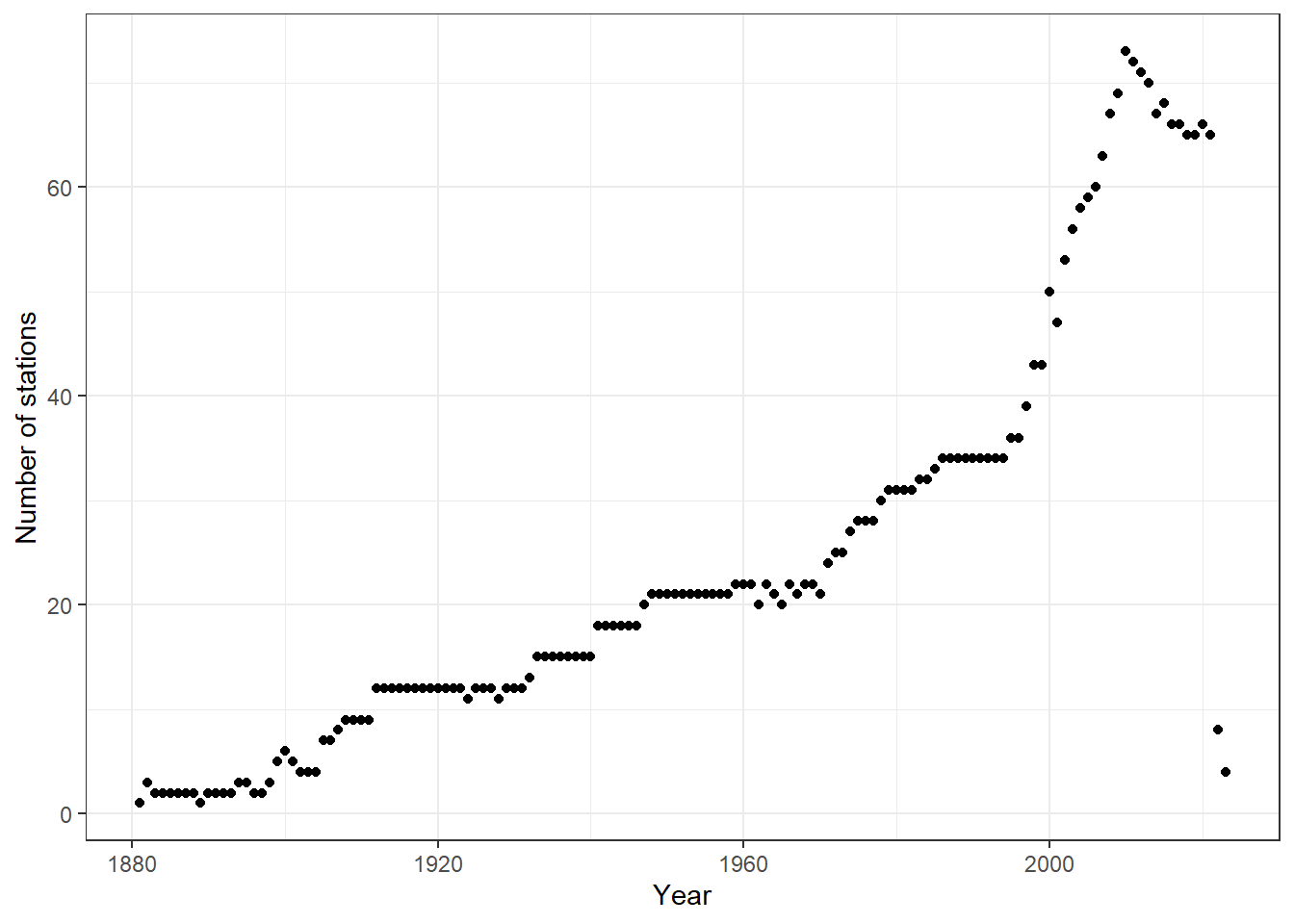

Calculate the response variables: Annual precipitation and January through April precipitation. We only keep the years that have 12 months of data.

precipitation_data<- monthlyPrecipData %>% 
              filter(!is.na(monthly_precip))%>%
              group_by(site, year)%>%filter(n() == 12)%>%
              summarize(annualPrecip = sum(monthly_precip, na.rm = TRUE),
              jfmaPrecip = sum(monthly_precip[month %in% c(1,2,3,4)], na.rm = TRUE))

Calculate long term averages per site

long_term_averages<-precipitation_data%>%group_by(site)%>%
summarize(longterm_mean_annual= mean(annualPrecip),longterm_mean_jfma=mean(jfmaPrecip))

How many years of actual data does every site has?

nyears= precipitation_data %>% filter(year>=1970 & year<=2016)%>%
 group_by(site) %>% tally() %>% 
 rename(nyears= n)%>% full_join(long_term_averages,by='site')

ggplot(nyears, aes(x = longterm_mean_annual, y = nyears)) +
  geom_point() +
  geom_text(aes(label = site), vjust = -0.5, size = 2) +
  labs(x = "Mean annual precipitation", y = "Number of Years")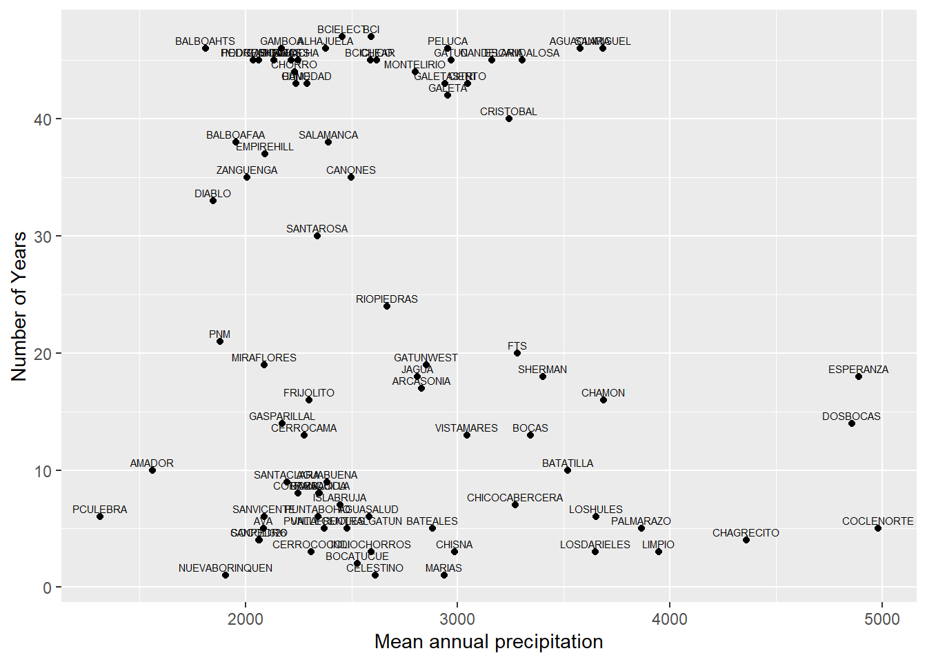

ggsave("plots/meanannual_v_nyears.jpg", width = 10, height = 6, dpi = 300)

Comment: we can clearly see a group of sites that has 30 or more years of data. Also, we recognize the presence of 3 sites with very high mean annual precipitation falling out of scope of our paper.

3.4 QAQC for sites

There is met stations located very close by to each other. We need to ensure that the set of data aren’t repeated.

An example is the Barro Colorado Island: which has 3 MET stations. Two of them are located within meters of each other. We will run some basic metrics to ensure this arent replicated stations.

BCI_subset<- precipitation_data%>% 
filter(site=="BCI"|site=="BCICLEAR"|site=="BCIELECT")%>%
filter(year>=1970 & year<=2016)

#test the differences between the three sets of data
means_BCI<-BCI_subset%>%group_by(site)%>%summarize(mean_annual_precip=mean(annualPrecip),sd_annual_precip=sd(annualPrecip),n=n())
anova_result <- aov(annualPrecip ~ site, data = BCI_subset)
tukey_results <- TukeyHSD(anova_result)

#ANOVA results
print(means_BCI)

# A tibble: 3 × 4
  site     mean_annual_precip sd_annual_precip     n
  <chr>                 <dbl>            <dbl> <int>
1 BCI                   2538.             590.    47
2 BCICLEAR              2649.             562.    45
3 BCIELECT              2292.             538.    47

summary(anova_result)

             Df   Sum Sq Mean Sq F value Pr(>F)   
site          2  3077427 1538713   4.842 0.0093 **
Residuals   136 43215268  317759                  
---
Signif. codes:  0 '***' 0.001 '**' 0.01 '*' 0.05 '.' 0.1 ' ' 1

print(tukey_results)

  Tukey multiple comparisons of means
    95% family-wise confidence level

Fit: aov(formula = annualPrecip ~ site, data = BCI_subset)

$site
                       diff       lwr       upr     p adj
BCICLEAR-BCI       110.2735 -168.3210 388.86788 0.6172843
BCIELECT-BCI      -245.9634 -521.5129  29.58622 0.0905150
BCIELECT-BCICLEAR -356.2368 -634.8312 -77.64239 0.0081833

ggplot(BCI_subset, aes(x=year, y=annualPrecip, color=site))+
geom_line()+theme_bw()+labs(x="Year", y="Annual Precipitation (mm)")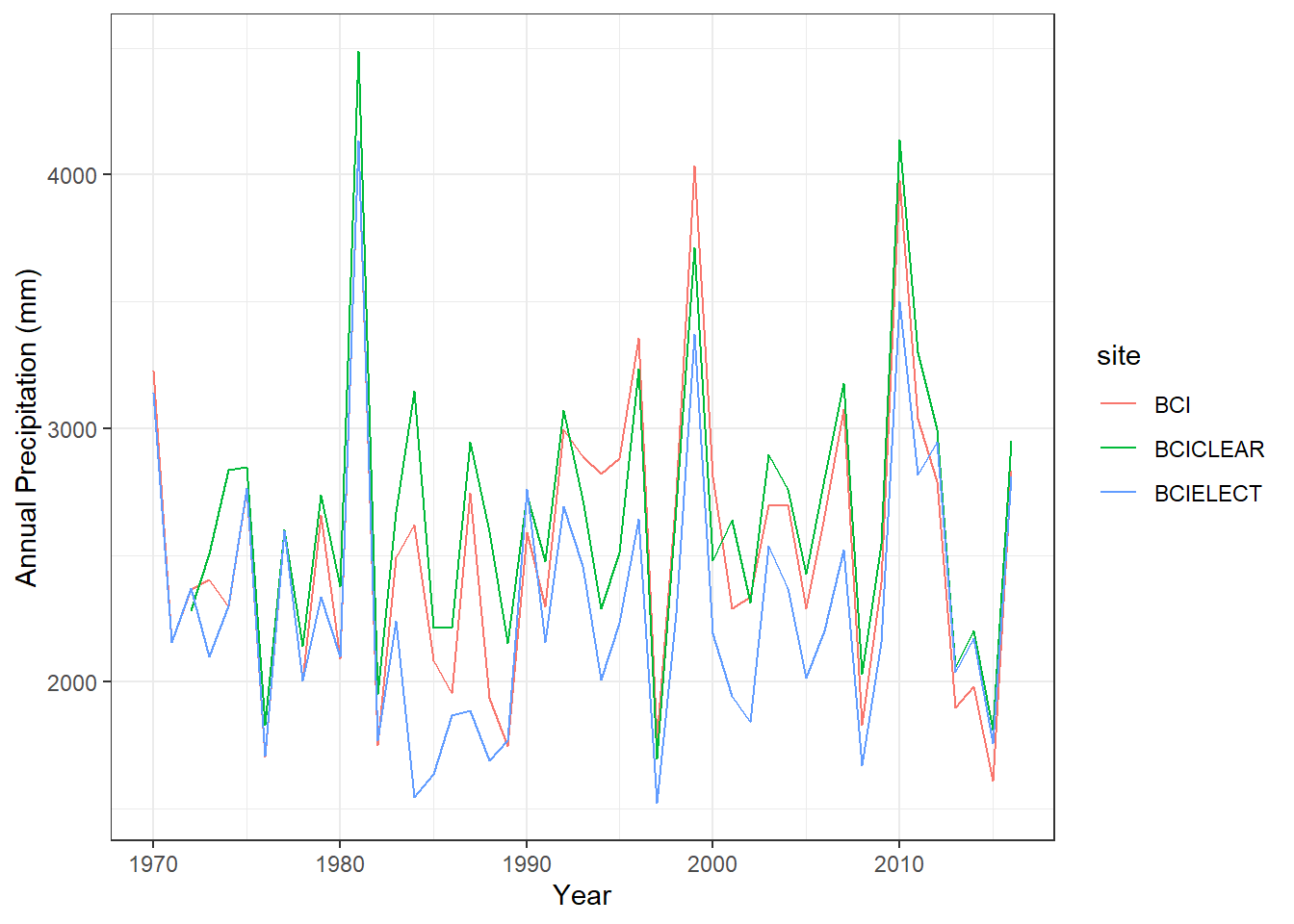

The metadata indicates that both BCICLEAR and BCIELECT are both different sensor. BCICLEAR is an standard rain gauge that is emptied manually by technicians. On the other hand, BCIELECT is a electronic tipping bucket showing 356 mm less annual mean precipitation. Finally, the BCI station managed by the Panama canal authority is placed on the Gatun lake shore. We will keep the three sites

The GALETA station appears on the ACP monthly summary and it is also listed in the STRI datasets, here given the name of GALETASTRI. Are this different sensors? or repeated sets of data.

#GALETA AND GALETASTRI
GALETA_subset<- precipitation_data%>% filter(site=="GALETA"|site=="GALETASTRI")%>%
filter(year>=1970 & year<=2016)
ggplot(GALETA_subset, aes(x=year, y=annualPrecip, color=site))+geom_line()+theme_bw()+labs(x="Year", y="Annual Precipitation (mm)")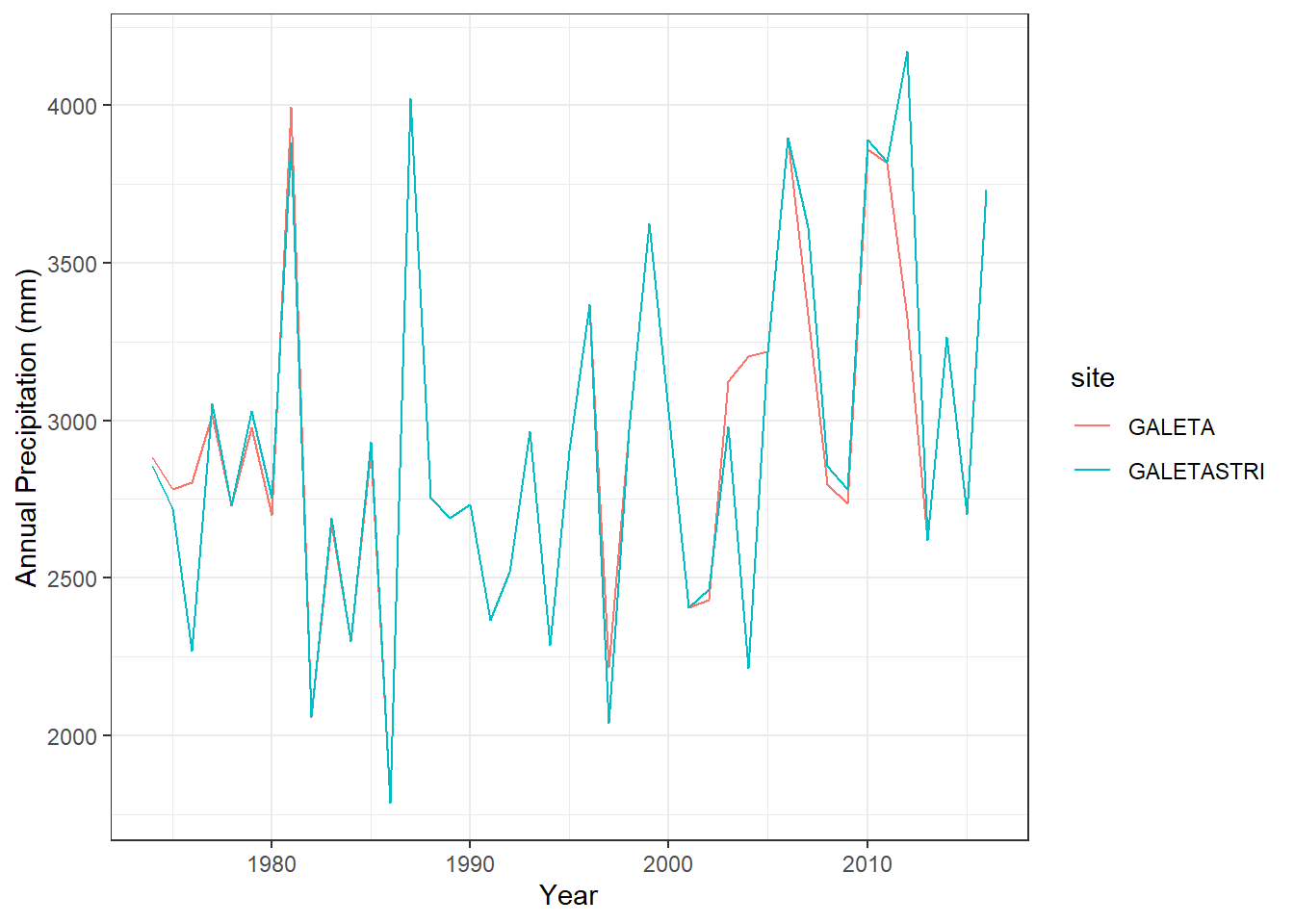

#anova
means_GALETA<-GALETA_subset%>%group_by(site)%>%summarize(mean_annual_precip=mean(annualPrecip),sd_annual_precip=sd(annualPrecip),n=n())
anova_galeta<- aov(annualPrecip ~ site, data = GALETA_subset)
tukey_results_galeta <- TukeyHSD(anova_galeta)

#ANOVA results
print(means_GALETA)

# A tibble: 2 × 4
  site       mean_annual_precip sd_annual_precip     n
  <chr>                   <dbl>            <dbl> <int>
1 GALETA                  2933.             533.    42
2 GALETASTRI              2930.             585.    43

summary(anova_galeta)

            Df   Sum Sq Mean Sq F value Pr(>F)
site         1      333     333   0.001  0.974
Residuals   83 26062365  314004               

print(tukey_results_galeta)

  Tukey multiple comparisons of means
    95% family-wise confidence level

Fit: aov(formula = annualPrecip ~ site, data = GALETA_subset)

$site
                       diff      lwr      upr     p adj
GALETASTRI-GALETA -3.957544 -245.751 237.8359 0.9741082

The GALETA case shows very little to no difference in the yearly averages for most of the years. The metadata of GALETASTRI mentions the use of Limon Bay to fill in the gaps and the Horizontal version of the ACP monthly summaries lists GALETA as ‘GALETA(STRI)’. We conclude that the sets of data are repeated. We will keep GALETASTRI since this monthly summaries were calculated in this study

Remove the GALETA station

precipitation_data_subset<- precipitation_data %>% filter(site!="GALETA") 

Filter the stations with more than 30 years of data between 1970 and 2016

precipitation_data_30<- merge(precipitation_data_subset, nyears, by.x= "site", by.y="site")
precipitation_data_subset<- precipitation_data_30%>% filter(nyears>=30)
unique(precipitation_data_subset$site)

 [1] "AGUACLARA"   "ALHAJUELA"   "BALBOAFAA"   "BALBOAHTS"   "BCI"        
 [6] "BCICLEAR"    "BCIELECT"    "CANDELARIA"  "CANO"        "CANONES"    
[11] "CASCADAS"    "CHICO"       "CHORRO"      "CIENTO"      "CRISTOBAL"  
[16] "DIABLO"      "EMPIREHILL"  "ESCANDALOSA" "GALETASTRI"  "GAMBOA"     
[21] "GATUN"       "GUACHA"      "HODGESHILL"  "HUMEDAD"     "MONTELIRIO" 
[26] "PEDROMIGUEL" "PELUCA"      "RAICES"      "SALAMANCA"   "SANMIGUEL"  
[31] "SANTAROSA"   "ZANGUENGA"  

3.5 Gap fill the timeseries 1970-2016

Use the lme4 package to fit a linear mixed model with random effects for year and fixed effects for site for annual precipitation and January to April precipitation (Bates et al. 2015). Note that we have created the model using all the avaliable years.

model_annual<- lmer(annualPrecip~ site +(1|year), data=precipitation_data_subset)
model_jfma<- lmer(jfmaPrecip~ site +(1|year), data=precipitation_data_subset)

We then filter the data to only the desired years.

precipitation_data_subset<- precipitation_data_subset%>%filter(year>=1970,year<=2016)

Create an empty data frame to predict the yearly and January through April precipitation.

year_sequence<- seq(1970,2016)
sites<- unique(precipitation_data_subset$site)
precipitation_predicted<- expand.grid(year_sequence,sites)%>%rename(year="Var1",site="Var2")

precipitation_predicted $predicted_annual<- predict(model_annual,newdata=precipitation_predicted)
precipitation_predicted$predicted_jfma<- predict(model_jfma,newdata=precipitation_predicted)

Gap fill the missing years using the predicted values to get a gap free time series.

precipitation<- precipitation_predicted %>%
full_join(precipitation_data_subset, by=c("site","year"))%>%
mutate(gap_fill=if_else(is.na(annualPrecip),TRUE,FALSE),
       annual=if_else(is.na(annualPrecip),predicted_annual,annualPrecip),
       jfma=if_else(is.na(jfmaPrecip),predicted_jfma,jfmaPrecip))

Whats the percentage of the data that is gap filled

gap_fill_true <- sum(precipitation$gap_fill == TRUE)
gap_fill_false <- sum(precipitation$gap_fill == FALSE)
percentage_gap_fill <- (gap_fill_true / (gap_fill_true + gap_fill_false)) * 100
percentage_gap_fill

[1] 9.175532

We can visualize subsets of the final precipitation data frame. Note that some sites will have more instances of predicted response variables.

ggplot(precipitation %>% filter(site %in% sites[1:8]), 
       aes(x = year, y = annual, group = site,color=site,shape=gap_fill)) + geom_line() + geom_point(size=3) +
  labs(x = "Year", y = "Annual Precipitation (mm)", color = "Site")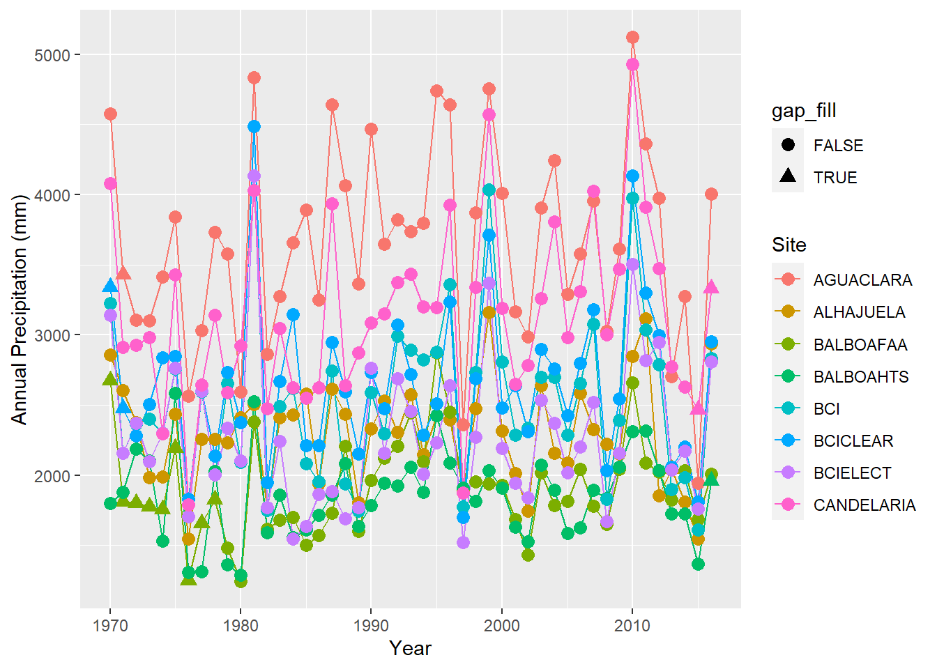

ggplot(precipitation %>% filter(site %in% sites[9:16]), 
       aes(x = year, y = annual, group = site,color=site,shape=gap_fill)) + geom_line() + geom_point(size=3) +
  labs(x = "Year", y = "Annual Precipitation (mm)", color = "Site")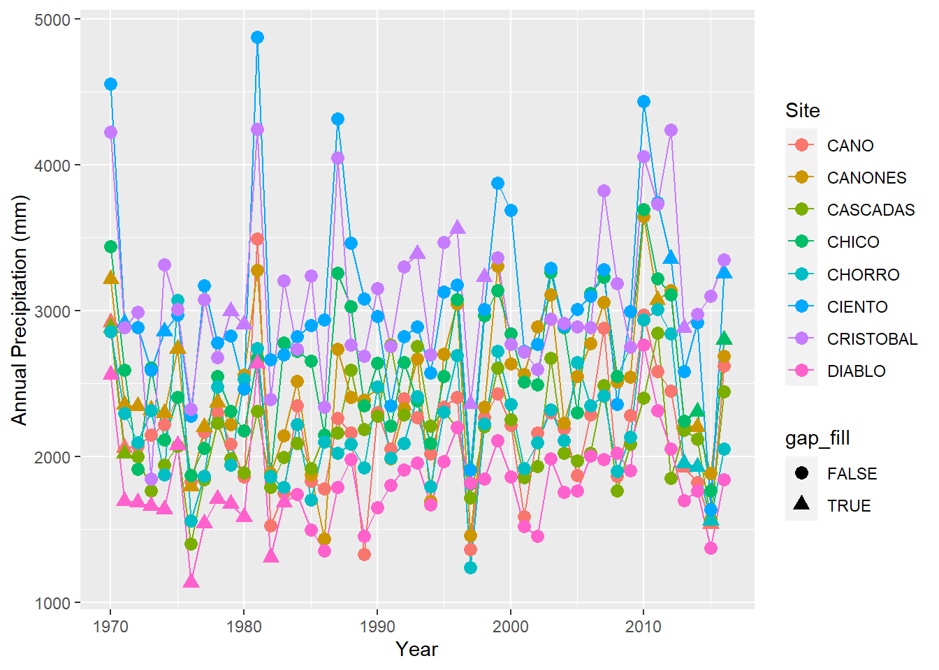

ggplot(precipitation %>% filter(site %in% sites[17:24]), 
       aes(x = year, y = annual, group = site,color=site,shape=gap_fill)) + geom_line() + geom_point(size=3) +
  labs(x = "Year", y = "Annual Precipitation (mm)", color = "Site")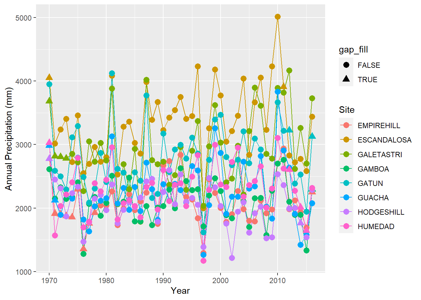

ggplot(precipitation %>% filter(site %in% sites[25:32]), 
       aes(x = year, y = annual, group = site,color=site,shape=gap_fill)) + geom_line() + geom_point(size=3) +
  labs(x = "Year", y = "Annual Precipitation (mm)", color = "Site")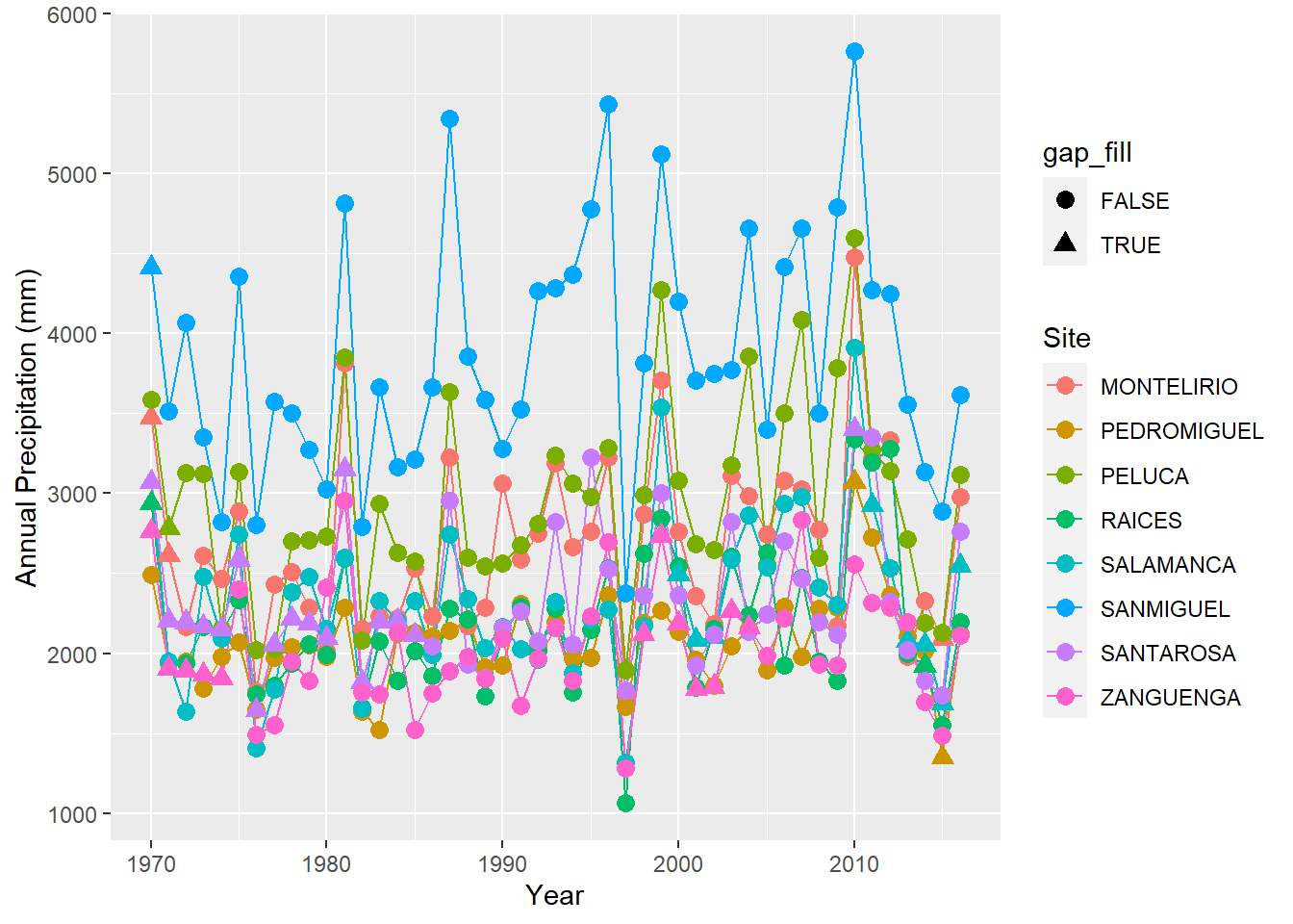

Finally, save the dataframe for its later use.

write.csv(precipitation,"../tables/precipitation.csv", row.names = FALSE)

Bates, Douglas, Martin Mächler, Ben Bolker, and Steve Walker. 2015. “Fitting Linear Mixed-Effects Models Using lme4.” Journal of Statistical Software 67 (1): 1–48. https://doi.org/10.18637/jss.v067.i01.